
Lorenzo Colli
“The present is the key to the past” is a oft-used phrase in the context of understanding our planet’s complex evolution. But this perspective can also be flipped, reflected, and reframed. In this Geodynamics 101 post, Lorenzo Colli, Research Assistant Professor at the University of Houston, USA, showcases some of the recent advances in modelling mantle convection.
Mantle convection is the fundamental process that drives a large part of the geologic activity at the Earth’s surface. Indeed, mantle convection can be framed as a dynamical theory that complements and expands the kinematic theory of plate tectonics: on the one hand it aims to describe and quantify the forces that cause tectonic processes; on the other, it provides an explanation for features – such as hotspot volcanism, chains of seamounts, large igneous provinces and anomalous non-isostatic topography – that aren’t accounted for by plate tectonics.
Mantle convection is both very simple and very complicated. In its essence, it is simply thermal convection: hot (and lighter) material goes up, cold (and denser) material goes down. We can describe thermal convection using classical equations of fluid dynamics, which are based on well-founded physical principles: the continuity equation enforces conservation of mass; the Navier-Stokes equation deals with conservation of momentum; and the heat equation embodies conservation of energy. Moreover, given the extremely large viscosity of the Earth’s mantle and the low rates of deformation, inertia and turbulence are utterly negligible and the Navier-Stokes equation can be simplified accordingly. One incredible consequence is that the flow field only depends on an instantaneous force balance, not on its past states, and it is thus time reversible. And when I say incredible, I really mean it: it looks like a magic trick. Check it out yourself.
With four parameters I can fit an elephant, and with five I can make him wiggle his trunk
This is as simple as it gets, in the sense that from here onward every additional aspect of mantle convection results in a more complex system: 3D variations in rheology and composition; phase transitions, melting and, more generally, the thermodynamics of mantle minerals; the feedbacks between deep Earth dynamics and surface processes. Each of these additional aspects results in a system that is harder and costlier to solve numerically, so much so that numerical models need to compromise, including some but excluding others, or giving up dimensionality, domain size or the ability to advance in time. More importantly, most of these aspects are so-called subgrid-scale processes: they deal with the macroscopic effect of some microscopic process that cannot be modelled at the same scale as the macroscopic flow and is too costly to model at the appropriate scale. Consequently, it needs to be parametrized. To make matters worse, some of these microscopic processes are not understood sufficiently well to begin with: the parametrizations are not formally derived from first-principle physics but are long-range extrapolations of semi-empirical laws. The end result is that it is possible to generate more complex – thus, in this regard, more Earth-like – models of mantle convection at the cost of an increase in tunable parameters. But what parameters give a truly better model? How can we test it?
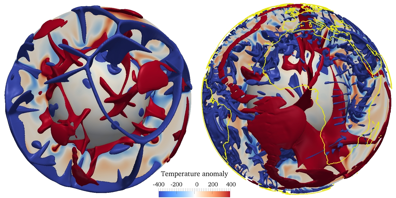
Figure 1: The mantle convection model on the left runs in ten minutes on your laptop. It is not the Earth. The one on the right takes two days on a supercomputer. It is fancier, but it is still not the real Earth.
Meteorologists face similar issues with their models of atmospheric circulation. For example, processes related to turbulence, clouds and rainfall need to be parametrized. Early weather forecast models were… less than ideal. But meteorologists can compare every day their model predictions with what actually occurs, thus objectively and quantitatively assessing what works and what doesn’t. As a result, during the last 40 years weather predictions have improved steadily (Bauer et al., 2015). Current models are better at using available information (what is technically called data assimilation; more on this later) and have parametrizations that better represent the physics of the underlying processes.
If time travel is possible, where are the geophysicists from the future?
We could do the same, in theory. We can initialize a mantle convection model with some best estimate for the present-day state of the Earth’s mantle and let it run forward into the future, with the explicit aim of forecasting its future evolution. But mantle convection evolves over millions of years instead of days, thus making future predictions impractical. Another option would be to initialize a mantle convection model in the distant past and run it forward, thus making predictions-in-the-past. But in this case we really don’t know the state of the mantle in the past. And as mantle convection is a chaotic process, even a small error in the initial condition quickly grows into a completely different model trajectory (Bello et al., 2014). One can mitigate this chaotic divergence by using data assimilation and imposing surface velocities as reconstructed by a kinematic model of past plate motions (Bunge et al., 1998), which indeed tends to bring the modelled evolution closer to the true one (Colli et al., 2015). But it would take hundreds of millions of years of error-free plate motions to eliminate the influence of the unknown initial condition.
As I mentioned before, the flow field is time reversible, so one can try to start from the present-day state and integrate the governing equations backward in time. But while the flow field is time reversible, the temperature field is not. Heat diffusion is physically irreversible and mathematically unstable when solved back in time. Plainly said, the temperature field blows up. Heat diffusion needs to be turned off [1], thus keeping only heat advection. This approach, aptly called backward advection (Steinberger and O’Connell, 1997), is limited to only a few tens of millions of years in the past (Conrad and Gurnis, 2003; Moucha and Forte, 2011): the errors induced by neglecting heat diffusion add up and the recovered “initial condition”, when integrated forward in time (or should I say, back to the future), doesn’t land back at the desired present-day state, following instead a divergent trajectory.
Per aspera ad astra
As all the simple approaches turn out to be either unfeasible or unsatisfactory, we need to turn our attention to more sophisticated ones. One option is to be more clever about data assimilation, for example using a Kalman filter (Bocher et al., 2016; 2018). This methodology allow for the combining of the physics of the system, as embodied by the numerical model, with observational data, while at the same time taking into account their relative uncertainties. A different approach is given by posing a formal inverse problem aimed at finding the “optimal” initial condition that evolves into the known (best-estimate) present-day state of the mantle. This inverse problem can be solved using the adjoint method (Bunge et al., 2003; Liu and Gurnis, 2008), a rather elegant mathematical technique that exploits the physics of the system to compute the sensitivity of the final condition to variations in the initial condition. Both methodologies are computationally very expensive. Like, many millions of CPU-hours expensive. But they allow for explicit predictions of the past history of mantle flow (Spasojevic & Gurnis, 2012; Colli et al., 2018), which can then be compared with evidence of past flow states as preserved by the geologic record, for example in the form of regional- and continental-scale unconformities (Friedrich et al., 2018) and planation surfaces (Guillocheau et al., 2018). The past history of the Earth thus holds the key to significantly advance our understanding of mantle dynamics by allowing us to test and improve our models of mantle convection.

Figure 2: A schematic illustration of a reconstruction of past mantle flow obtained via the adjoint method. Symbols represent model states at discrete times. They are connected by lines representing model evolution over time. The procedure starts from a first guess of the state of the mantle in the distant past (orange circle). When evolved in time (red triangles) it will not reproduce the present-day state of the real Earth (purple cross). The adjoint method tells you in which direction the initial condition needs to be shifted in order to move the modeled present-day state closer to the real Earth. By iteratively correcting the first guess an optimized evolution (green stars) can be obtained, which matches the present-day state of the Earth.
1.Or even to be reversed in sign, to make the time-reversed heat equation unconditionally stable.