Seismologists work hard to provide the best snapshots of the Earth’s mantle. Yet tomographic models based on different approaches or using different data sets sometimes obtain quite different details. It is hard to know for a non specialist if small scale anomalies can be trusted and why. This week Maria Koroni and Daniel Bowden, both postdocs in the Seismology and Wave Physics group in ETH Zürich, tell us how these beautiful images of the Earth are obtained in practice.

Daniel Bowden and Maria Koroni enjoying coffee in Zürich
Seismology is a science that aims at providing tomographic images of the Earth’s interior, similar to X-ray images of the human body. These images can be used as snapshots of the current state of flow patterns inside the mantle. The main way we communicate, from tomographer to geodynamicist, is through publication of some tomographic image. We seismologists, however, make countless choices, approximations and assumptions, which are limited by poor data coverage, and ultimately never fit our data perfectly. These things are often overlooked, or taken for granted and poorly communicated. Inevitably, this undermines the rigour and usefulness of subsequent interpretations in terms of heat or material properties. This post will give an overview of what can worry a seismologist/tomographer. Our goal is not to teach seismic tomography, but to plant a seed that will make geodynamicists push seismologists for better accuracy, robustness, and communicated uncertainty!
A typical day in a seismologist’s life starts with downloading some data for a specific application. Then we cry while looking at waveforms that make no sense (compared to the clean and physically meaningful synthetics calculated the day before). After a sip, or two, or two thousand sips of freshly brewed coffee, and some pre-processing steps to clean up the mess that is real data, the seismologist sets up a measurement of the misfit between synthetics and observed waveforms. Do we try to simulate the entire seismogram, just its travel time, its amplitude? The choice we make in defining this misfit can non-linearly affect our outcome, and there’s no clear way to quantify that uncertainty.
After obtaining the misfit measurements, the seismologist starts thinking about best inversion practices in order to derive some model parameters. There are two more factors to consider now: how to mathematically find a solution that fits our data, and the choice of how to choose a subjectively unique solution from the many solutions of the problem… The number of (quasi-)arbitrary choices can increase dramatically in the course of the poor seismologist’s day!
The goal is to image seismic anomalies; to present a velocity model that is somehow different from the assumed background. After that, the seismologist can go home, relax and write a paper about what the model shows in geological terms. Or… More questions arise and doubts come flooding in. Are the choices I made sensible? Should I make a calculation of the errors associated with my model? Thermodynamics gives us the basic equations to translate seismic to thermal anomalies in the Earth but how can we improve the estimated velocity model for a more realistic interpretation?
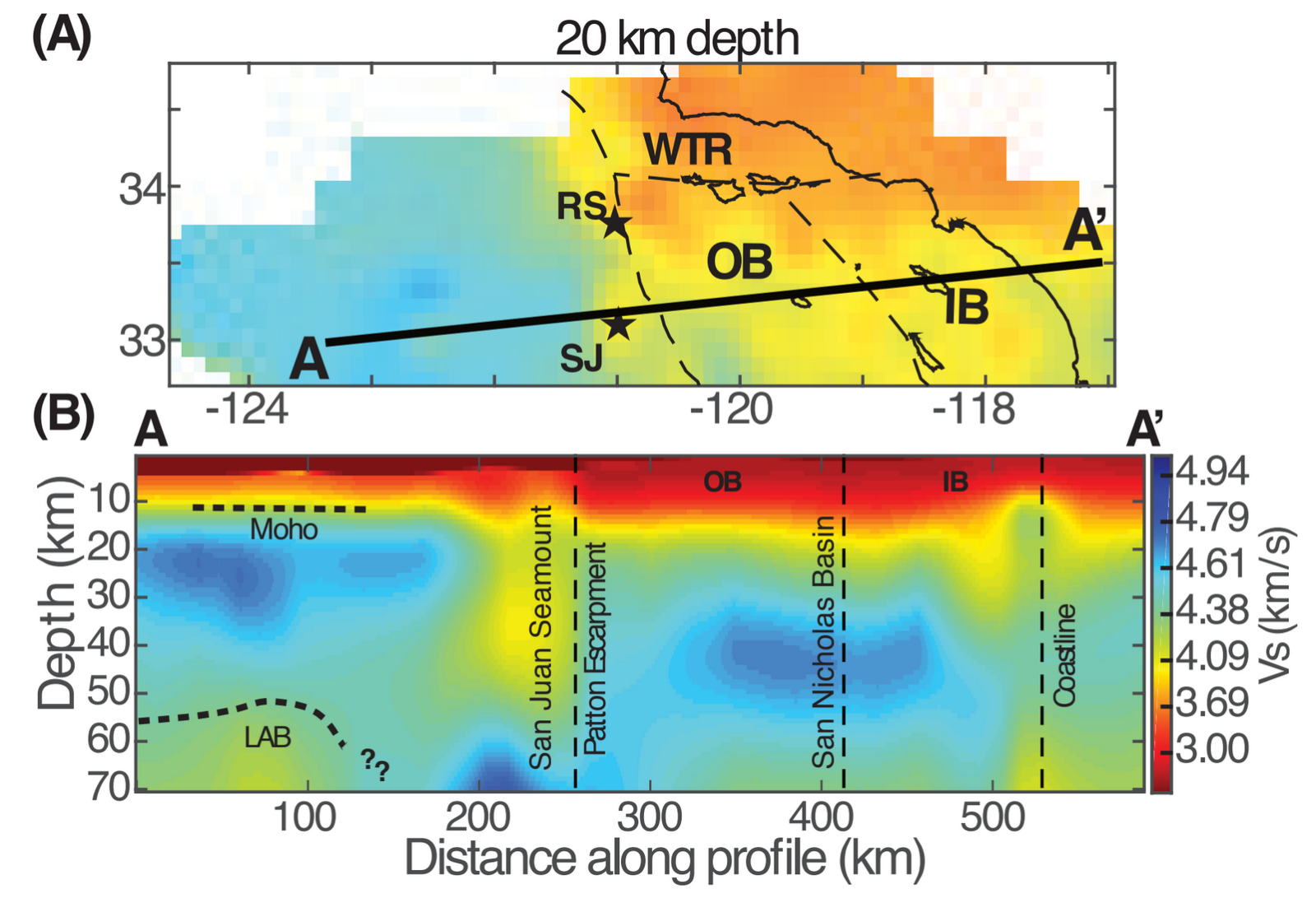
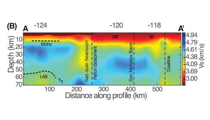
Figure 1: A tomographic velocity model, offshore southern California. What do the blobs mean? This figure is modified from the full paper at https://doi.org/10.1002/2016JB012919
Figure 1 is one such example of a velocity model, constructed through seismic tomography (specifically from ambient-noise surface waves). The paper reviews the tectonic history of the crust and upper mantle in this offshore region. We are proud of this model, and sincerely hope it can be of use to those studying tectonics or dynamics. We are also painfully aware of the assumptions that we had to make, however. This picture could look drastically different if we had used a different amount of regularization (smoothing), had made different prior assumptions about where layers may be, had been more or less restrictive in cleaning our raw data observations, or made any number of other changes. We were careful in all these regards, and ran test after test over the course of several months to ensure the process was up to high standards, but for the most part… you just have to take our word for it.
There’s a number of features we interpret here: thinning of the crust, upwelling asthenosphere, the formation of volcanic seamounts, etc. But it wouldn’t shock me if some other study came out in the coming years that told an entirely different story; indeed that’s part of our process as scientists to continue to challenge and test hypotheses. But what if this model is used as an input to something else as-of-yet unconstrained? In this model, could the Lithosphere-Asthenosphere Boundary (LAB) shown here be 10 km higher or deeper, and why does it disappear at 200km along the profile? Couldn’t that impact geodynamicists’ work dramatically? Our field is a collaborative effort, but if we as seismologists can’t properly quantify the uncertainties in our pretty, colourful models, what kind of effect might we be having on the field of geodynamics?
Another example comes from global scale models. Taking a look at figures 6 and 7 in Meier et al. 2009, ”Global variations of temperature and water content in the mantle transition zone from higher mode surface waves” (DOI:10.1016/j.epsl.2009.03.004), you can observe global discontinuity models and you are invited to notice their differences. Some major features keep appearing in all of them, which is encouraging since it shows that we may be indeed looking at some real properties of the mantle. However, even similar methodologies have not often converged to same tomographic images. The sources of discrepancies are the usual plagues in seismic tomography, some of them mentioned on top.
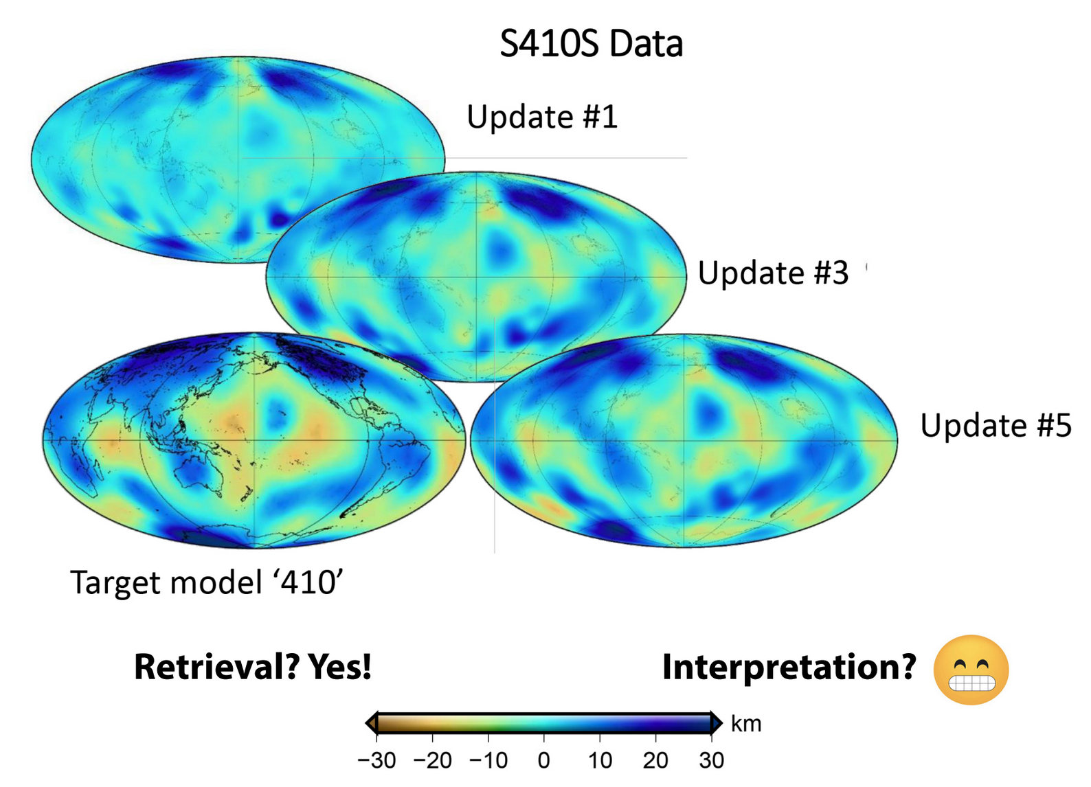
Figure 2: Global models of the 410 km discontinuity derived after 5 iterations using traveltime data. We verified that the method retrieves target models almost perfectly. Data can be well modelled in terms of discontinuity structure; but how easily can they be interpreted in terms of thermal and/or compositional variations?
In an effort to improve imaging of mantle discontinuities, especially those at 410 and 660 km depths which are highly relevant to geodynamics (I’ve been told…), we have put some effort into building up a different approach. Usually, traveltime tomography and one-step interpretation of body wave traveltimes have been the default for producing images of mantle transition zone. We proposed an iterative optimisation of a pre-existing model, that includes flat discontinuities, using traveltimes in a full-waveform inversion scheme (see figure 2). The goal was to see whether we can get the topography of the discontinuities out using the new approach. This method seems to perform very well and it gives the potential for higher resolution imaging. Are my models capable of resolving mineralogical transitions and thermal variations along the depths of 410 and 660 km?
The most desired outcome would be not only a model that represents Earth parameters realistically but also one that provides error bars, which essentially quantify uncertainties. Providing error bars, however, requires extra computational work, and as every pixel-obsessed seismologist, we would be curious to know the extent to which uncertainties are useful to a numerical modeller! Our main question, then, remains: how can we build an interdisciplinary approach that can justify large amounts of burnt computational power?
As (computational) seismologists we pose questions for our regional or global models: Are velocity anomalies good enough, intuitively coloured as blue and red blobs and representative of heat and mass transfer in the Earth, or is it essential that we determine their shapes and sizes with greater detail? Determining a range of values for the derived seismic parameters (instead of a single estimation) could allow geodynamicists to take into account different scenarios of complex thermal and compositional patterns. We hope that this short article gave some insight into the questions a seismologist faces each time they derive a tomographic model. The resolution of seismic models is always a point of vigorous discussions but it could also be a great platform for interaction between seismologists and geodynamicists, so let’s do it!
For an overview of tomographic methodologies the reader is referred to Q. Liu & Y. J. Gu, Seismic imaging: From classical to adjoint tomography, 2012, Tectonophysics. https://doi.org/10.1016/j.tecto.2012.07.006