
Luke Mondy
The Geodynamics 101 series serves to showcase the diversity of research topics and methods in the geodynamics community in an understandable manner. We welcome all researchers – PhD students to Professors – to introduce their area of expertise in a lighthearted, entertaining manner and touch upon some of the outstanding questions and problems related to their fields. For our latest ‘Geodynamics 101’ post, PhD candidate Luke Mondy from the EarthByte Group at the University of Sydney blogs about some impressively high-resolution numerical models of ‘rotational rifting,’ and the role of gravity. Luke also shares a bit about the journey behind this work, which recently appeared in Geology.
In geodynamic modelling, we’re always thinking about forces. It’s a balancing act of plate driving forces potentially interacting with the upwelling mantle, or maybe sediment loading, or thermal relaxation… the list goes on.
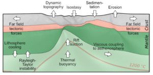
Figure 1: A summary of the forces interacting during continental rifting, from Brune, 2018.
But the thing that underpins all of these forces, fundamentally, is our favourite but oft forgotten force: gravity. Here, I’ll tell the story of investigating a numerical model of continental rifting and discovering – or rather, rediscovering – the importance of gravity as a fundamental force in driving Earth dynamics.
How it started – a side project!
A few years ago, my colleagues and I were granted access to not just one, but two, big supercomputers in Australia: Raijin, and Magnus. Both were brand new and raring to go – but we needed something big to test them out on. At the time, 3D geodynamic models were typically limited to quite low resolution, since they can be so computationally demanding, but since we had access to this new power, we decided to see how far we could push the computers to address a fundamentally 3D problem.
2D vs 3D
Historically, subduction and rifting have been ideal settings to model as they can be constrained to two dimensions while still retaining most of their characteristic properties.
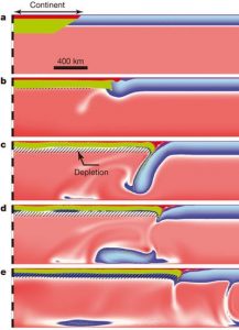
Figure 2. A 2D subduction model. Despite being ‘only’ two dimensions, the fundamental and interesting aspects of the problem are still captured by the model. Figure from Rey et al., 2014.
However, as tremendously useful as these models have been, many interesting problems in geodynamics are fundamentally three dimensional. The obvious example is global mantle convection, but we are starting to see more and more papers addressing both rifting and subduction problems that require 3D contexts, for example: continental accretion (Moresi et al., 2014), metamorphic core complex formation (Rey et al., 2017), or oblique rifting (Brune et al., 2012).
Typically when we model a rift in 2D, the dimensionality implies that we are looking at orthogonal rifting – that the plates move away from each other perpendicular to the rift axis. Since 2D models cannot account for forces in the third dimension, they are only suitable for when the applied tectonic forces pull within the plane of the model – that is, when the 2D model lies along a small circle of an Euler pole.
Euler poles have another interesting geometric property – the velocity of extension between two plates changes as we move closer or further away from the Euler pole: zero velocity at the pole itself, and fastest at the equator to the pole (Lundin et al., 2014).
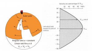
Figure 3. Left: From Lundin et. al. (2014), the figure shows the geometric relationship of increasing rifting velocity as the distance from the pole increases. Right: the same relationship graphed out, showing the cosine curve (Kearey et.al. 2009).
This leads to differing extension velocities along the length of the rift axis. Extension velocities are a huge control on the resulting geodynamics (e.g., Buck et al., 1999). Employing a series of 2D models along a rift axis (Brune et al., 2014) has been used to show how these dynamics change, but misses out on the three-dimensionality of the problem – how do these differing and diachronous dynamics interact with each along other the rift margin as it forms?
Rotational Rifting
We decided to attempt to model this sort of rifting, as we termed it “rotational rifting”. Essentially we linked up the 2D slices along the rift axis into one big 3D model – so that we have slow extension towards the Euler pole, and fast extension away from it.
To do this, we ended up using the code Underworld (at the time version 1.8 – but their 2.0 version is the best place to start!), and a framework developed inside the EarthByte group at the University of Sydney called the ‘Lithospheric Modelling Recipe’, or LMR.
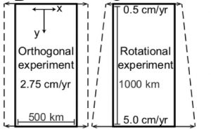
Figure 4. Map view of the two experiments. Arrows show the velocity boundary conditions applied. Note they are perpendicular to the model domain – we thought long and hard about this choice, and explain it fully in the Data Repository.
Using the LMR, we set up two 3D experiments: both are 1000 km by 500 km along the surface, and 180 km deep. The ‘orthogonal’ experiment is modelled at the equator to the pole – so the velocities along the walls are the same all the way along the rift axis. The ‘rotational’ experiment is very close to the Euler pole (where the rate of extension velocity change is greatest), from 89 degrees to 79 degrees (90 degrees being the Euler pole), which gives an imposed velocity at the slow end (89 degrees) of 0.5 cm/yr and at the fast end (79 degrees) 5.0 cm/yr.
Since we wanted to stress test the supercomputers, we ran these experiments at just under 2 km grid resolution (256 x 512 x 96). This meant each experiment ended up using about 2.5 billion particles to track the materials! The 2 km grid size is an important milestone – to properly resolve faulting, sub-2 km grid sizes are required (Gerya, 2009).
The results!
So we ran the experiments, and compared the results! To give a broad overview of what we found, here’s a nice animation:

Figure 5. Top: Animation showing the orthogonal experiment from a south-west perspective (with the Euler pole being the ‘north’ pole). The light grey layers show the upper crust, dark grey the lower crust. Half of the crust has been removed to show the lithospheric mantle topography. The blue to the white colours show the lithospheric mantle temperature, and from white to red shows the asthenospheric temperature. Bottom: As above but for the rotational experiment. Notice that the asthenospheric dome migrates along the rift towards the Euler pole.
What to do now?
Cool looking experiments, of course! The supercomputers had been able to handle the serious load we put on them (it took about 2 weeks per experiment, on ~800 cpus), so that part of the project was a success. But what about the experiments themselves – did switching to 3D actually tell us anything useful?
What we expected…
The things we expected were there. The orthogonal experiment behaved identically to a 2D model. For the rotational experiment, we found the style of faulting changed and evolved along the rift axis, and seemed to match up nicely with the 2D work about differing extension rates. We were able to identify phases of rifting via strain patterns, which were similar to those described by Lavier and Manatschal (2006), and seemed to match the outputs of the series of 2D models along a rift axis.
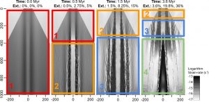
Figure 6. Map view of strain-rate of the rotational experiment through time. The phases (1 through 4, representing different modes of deformation) migrate along the rift towards the Euler pole.
What we didn’t expect…
Almost on a whim, we decided to start looking into the tectonic regime. Using the visualization program Paraview, we calculated the eigenvectors of the deviatoric stress and assigned a tectonic regime (blue for extension, red for compression, green for strike-slip, and white for undetermined), following a similar scheme to the World stress map (Zoback, 1992). Apologies to colour blind folk!
Here’s what a selected section of the orthogonal experiment surface looks like through time:
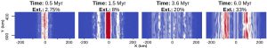 Figure 7. The stress regimes at the surface of the orthogonal experiment (clipped to y = ~400 to ~600 km).
Not really that surprising – we found mostly extension everywhere, with a bit of compression when the central graben sinks down and gets squeezed. However, it was a little bit surprising to see the compression come back on the rift flanks.
But when we applied the same technique to the rotational experiment, we found this on the surface:
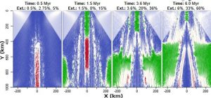
Figure 8. The stress regimes at the surface of the rotational experiment. The three numbers at the top represent the total extension at y = 0 km, 500 km, and 1000 km respectively.
Now all of a sudden we’re seeing strike-slip stress regimes in different areas of the experiment!
The above figures displaying the stress in the experiments so far have been of the surface – where one of the principal stress axes must be vertical – but our colouring technique does not limit us to just the surface. We noticed when looking at cross-sections that the lithospheric mantle was also showing unexpected stress regimes!
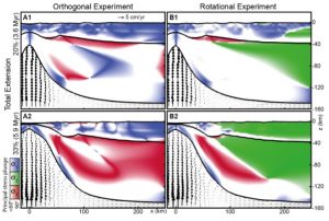
Figure 9. Slices at y = 500 km across the rift axis (right in the middle). Coloured areas show where the plunge of one principal stress axis is >60 degrees. Both experiments have the same applied extension velocity at y = 500 km, and so total extension is equivalent between experiments.
In most of the lithosphere, the strain rate is still very small, not enough to notice much deformation (1e-16 to 1e-18 1/s). But a few puzzling questions were raised: why do we see compressional tectonic regimes in the orthogonal experiment; and why do we also see strike-slip regimes in the rotational experiment?
Gravitational Potential Energy (GPE)
It quickly became apparent that these stress changes were related to the upwelling asthenosphere, as the switch between regimes was well timed to when the asthenosphere would approach the Moho – about 40 km depth. This gave us the hint that perhaps buoyancy forces were at play. We used Paraview again to calculate the gravitational potential energy at each point on the surface (taking into account all the temperature dependent densities, detailed topography, and so on), and produced these maps:
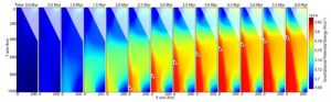
Figure 10. A time series showing the gravitational potential energy (GPE) at each point on the surface of the rotational experiment. Only half the surface is shown because it is symmetrical. The small triangle notch is where we determined the rift tip to be located (where 1/(beta factor) < 0.2).
What we saw confirmed our suspicions – the rise of the asthenospheric dome induces a gravitational force that radiates outwards. The juxtaposition of the hot, yet still quite heavy, asthenospheric material, next to practically unthinned crust on both the rift flanks and ahead of the rift tip, produces a significant force.
But why the switch to compression or strike-slip tectonic regimes in an otherwise extensional setting? In the case of the orthogonal model, the force (aka the difference in GPE) is perpendicular to the rift axis, since the dome rises synchronously along the axis. When this force overcomes the far-field tectonic force (essentially the force required to drive our experiment boundary conditions), the stress regime changes from extension to compression.
However, in the rotational experiment, the dome is larger the further away from the Euler pole, and so instead the gravitational force radiates outwards from the dome. Now the stress in the lithospheric mantle has to deal with not only the force induced from the upwelling asthenosphere right next to it, but also from along the rift axis (have a look at the topography of the lithospheric mantle in Fig. 5). These combined forces end up rotating the principal stresses such that sigma_2 stands vertical and a strike-slip regime is generated.
We also see the gravitational force manifest in other ways. Looking at the along axis flow in the asthenosphere, the experiment initially predicts a suction force towards the rapidly opening end of the model (away from the Euler pole), similar to Koopmann et al. (2014). But once the dome is formed, we see a reversal of this flow, back towards the Euler pole, driven by gravitational collapse. This flow appears to apply a strong stress to the crust surrounding the dome, reaching upwards of 50 MPa in some places.
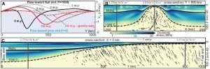
Figure 11. A: The direction of flow at the lithosphere-asthenosphere boundary in the centre of the rift. Early in the experiment, we see suction towards the fast end of the rift, while later in the experiment, we see a return flow. The dashed line shows the flow after the tectonic boundary conditions have been removed. B,C: cross-sections showing stress and velocity arrows from the experiment just after the tectonic boundary conditions have been removed.
How do we know it’s gravity?
To test this idea further, we ran some additional experiments. First, we let the rotational experiment run for about 3.6 Million years, and then ‘stopped’ the tectonics (changed the side velocity boundary conditions to 0 cm/yr) – leaving gravity as the only driving force. We saw that the return flow towards the Euler pole was still present (though reduced). By running some more rotational experiments with either doubled or halved Euler pole rotational rate, we saw that the initial suction magnitude correlates with the change in opening velocity, but the return flow to the Euler pole is almost identical, giving further evidence that this is gravity driven.
What about the real world?
We numerical modellers love to stay in the world of numbers – but alas sometime we must get our hands dirty and look at the real world – just to make sure our models actually tell us something useful!
Despite our slightly backwards methodology (model first, check nature second), it did give us an advantage: our experiments were producing predictions for us to go and test. We had our hypothesis – now to see if it could be validated.
So we went out and looked for examples of rifting near an Euler pole, and the two most notable we found were in the Woodlark Basin, Papua New Guinea, and the Galapagos Rise in the Pacific. Despite the ‘complications’ of the natural world (things like sediment loading, pre-existing weakness in the crust, etc. – things that get your hands dirty), we found a striking first order relationship between the earthquake focal mechanisms present in both areas, and what our experiments predicted:
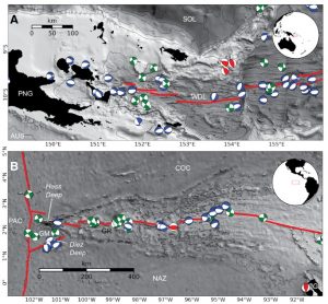
Figure 12. Top: the Woodlark Basin, PNG. Bottom: the Galapagos Rise. Both show earthquake focal mechanisms, coloured the same way as our experiments: blue for extension, red for compression, and green for strike-slip.
Furthermore, much work has been done investigating the Hess deep, a depression that sits ahead of the rift tip in the Galapagos. We found in our rotational experiment a similar ‘deep’ that moves ahead of the rift tip through time, giving us greater confidence in our experimental predictions.
Takeaways
There are a few things I’ve taken away from this experience. The first is that it’s important to remember the fundamentals. I’ve found that, generally, geodynamicists initially think about the force-balances going on in a particular setting, but gravity was staring me in the face for a while before I understood its critical role.
The second take-away was that exploratory modelling – playing around with experiments just for fun – is a great thing to do. Probably most of us do this anyway as part of the day-to-day activities, but putting aside some time to think about what sort of things to try out allowed us to find something really interesting. Furthermore, we then had a whole host of predictions we could go out and look for, rather than trying to tweak out experiment parameters to match something we already had found.
Finally, the 3D revolution we’re going through at the moment is exciting! Now that there are computers available to us that are able to run these enormous calculations, it gives us a chance to explore these fundamental problems in a new way and hopefully learn something about the world!
If you would like to checkout our paper, you can see it here. We made all of our input files open-source (and the code Underworld is already open-source), so please check them out too!
References

Brune, S., Popov, A. A., & Sobolev, S. V. (2012). Modeling suggests that oblique extension facilitates rifting and continental break‐up. Journal of Geophysical Research: Solid Earth, 117(B8).

Brune, S., Heine, C., Pérez-Gussinyé, M., & Sobolev, S. V. (2014). Rift migration explains continental margin asymmetry and crustal hyper-extension. Nature Communications, 5, 4014.

Brune, S. (2018). Forces within continental and oceanic rifts: Numerical modeling elucidates the impact of asthenospheric flow on surface stress. Geology, 46(2), 191-192.

Buck, W. R., Lavier, L. L., & Poliakov, A. N. (1999). How to make a rift wide. Philosophical Transactions - Royal Society of London Series A, Mathematical Physical and Engineering Sciences, 671-689.

Gerya, T. (2009). Introduction to numerical geodynamic modelling. Cambridge University Press.

Kearey, P. (Ed.). (2009). The Encyclopedia of the solid earth sciences. John Wiley & Sons.

Lundin, E. R., Redfield, T. F., Péron-Pindivic, G., & Pindell, J. (2014, January). Rifted continental margins: geometric influence on crustal architecture and melting. In Sedimentary Basins: Origin, Depositional Histories, and Petroleum Systems. 33rd Annual GCSSEPM Foundation Bob F. Perkins Conference. Gulf Coast Section SEPM (GCSSEPM), Houston, TX (pp. 18-53).

Koopmann, H., Brune, S., Franke, D., & Breuer, S. (2014). Linking rift propagation barriers to excess magmatism at volcanic rifted margins. Geology, 42(12), 1071-1074.

Lavier, L. L., & Manatschal, G. (2006). A mechanism to thin the continental lithosphere at magma-poor margins. Nature, 440(7082), 324.

Mondy, L. S., Rey, P. F., Duclaux, G., & Moresi, L. (2018). The role of asthenospheric flow during rift propagation and breakup. Geology.

Moresi, L., Betts, P. G., Miller, M. S., & Cayley, R. A. (2014). Dynamics of continental accretion. Nature, 508(7495), 245.

Rey, P. F., Coltice, N., & Flament, N. (2014). Spreading continents kick-started plate tectonics. Nature, 513(7518), 405.

Rey, P. F., Mondy, L., Duclaux, G., Teyssier, C., Whitney, D. L., Bocher, M., & Prigent, C. (2017). The origin of contractional structures in extensional gneiss domes. Geology, 45(3), 263-266.

Zoback, M. L. (1992). First‐and second‐order patterns of stress in the lithosphere: The World Stress Map Project. Journal of Geophysical Research: Solid Earth, 97(B8), 11703-11728.