
Inverse theory exists to make the life of the mantle geodynamicist easier.
The Geodynamics 101 series serves to showcase the diversity of research topics and methods in the geodynamics community in an understandable manner. We welcome all researchers – PhD students to professors – to introduce their area of expertise in a lighthearted, entertaining manner and touch upon some of the outstanding questions and problems related to their fields. This time, Lars Gebraad, PhD student in seismology at ETH Zürich, Switzerland, talks about inversion and how it can be used in geodynamics! Due to the ambitious scope of this topic, we have a 3-part series on this! You can find the first post here. This week, we have our second post in the series, where Lars discusses the inverse problem and deterministic inversion.
 The idea of inversion is to literally invert the forward problem. For the aforementioned problems our knowns become unknowns, and vice versa. We wish to infer physical system parameters from measurements. Note that in our forward problem there are multiple classes of knowns; we have the forcing parameters, the material properties and the boundary conditions. All of these parameters could be inverted for in an inversion, but it is typically one only inverts for one class. Most of the time, medium parameters are the target of inversions. As we will go through the examples, I will gradually introduce some inversion methods. Every new method is marked in blue.
Estimating ingredients from a bread
Now, let’s consider our first example: the recipe for a bread. Let’s say we have a 0.5 kilogram bread. For our first case (case 1a), we will assume that the amount of water is ideal. In this case, we have one free variable to estimate (the used amount of flour), from one observable (the resulting amount of bread). We have an analytical relationship that is both invertible and one-to-one. Therefore, we can use the direct inversion of the relationship to compute the amount of flour. The process would go like this:
Direct inversion
1. Obtain the forward expression G(m) = d;
2. Solve this formula for G^-1 (d) = m;
3. Find m by plugging d into the inverse function.
Applying this direct inversion shows us that 312.5 grams of flour must have been used.
The two properties of the analytical relationship (invertible and one-to one) are very important for our choice of this inversion method. If our relationship was sufficiently complex, we couldn’t solve the formula analytically (though the limitation might then lie by the implementer 😉 ). If a function is not one-to-one, then two different inputs could have the same output, so we cannot analytically invert for a unique solution.
In large linear forward models (as often obtained in finite difference and finite element implementations), we have a matrix formula similar to
A m = d.
In these systems, m is a vector of model parameters, and d a vector of observables. If the matrix is invertible, we can directly obtain the model parameters from our observables. The invertibility of the matrix is a very important concept, which I will come back to in a bit.
Problems in direct inversion, misfits and gradient descents
Let’s see what happens when the first condition is not satisfied. I tried creating a non-linear function that at least I could not invert. Someone might be able to do it, but that is not the aim of this exercise. This new relationship is given here:
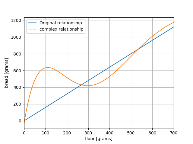
Complex flour to bread relationship, another 1D forward model.
The actual forward model is included in the script at the bottom of the post. When we cannot analytically solve the forward model, one approach would be to iteratively optimise the input parameters such that the end result becomes as close as possible to the observed real world. But, before we talk about how to propose inputs, we need a way to compare the outputs of our model to the observables!
When we talk about our bread, we see one end-product. It is very easy to compare the result of our simulation to the real world. But what happens when we make a few breads, or, similarly, when we have a lot of temperature observations in our volcanic model? One (common) way to combine observables and predictions into a single measure of discrepancy is by defining a misfit formula which takes into account all observations and predictions, and returns a single – you guessed it – misfit.
The choice of misfit directly influences which data is deemed more important in an inversion scheme, and many choices exist. One of the most intuitive is the L2-norm (or L2 misfit), which calculates the vector distance between the predicted data (from our forward model) with the observed data as if in Euclidean space. For our bread it would simply be
X = | predicted bread – observed bread |
Let’s try to create a misfit function for our 1D bread model. I use the relationship in the included scripts. Again, we have 500 grams of bread. By calculating the quantity | G(m) – 500 |, we can now make a graph of how the misfit varies as we change the amount of flour. I created a figure which shows the observed and predicted value:
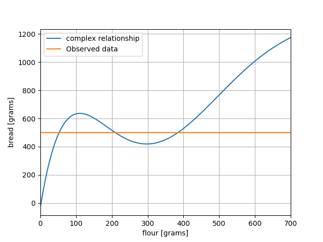
Complex flour to bread relationship with observation superimposed
and a figure which shows the actual misfit at each value of m

Misfit between model and observation
Looking at the two previous figures may result in some questions and insights to the reader. First and foremost, it should be obvious that this problem does not have a unique solution. Different amounts of flour give exactly the same end result! It is thus impossible to say with certainty how much flour was used.
We have also recast our inversion problem as an optimisation function. Instead of thinking about fitting observations we can now think of our problem as a minimization of some function X (the misfit). This is very important in inversion.
Iterative optimizations schemes such as gradient descent methods (and the plethora of methods derived from it) work in the following fashion:
Gradient descent inversion/optimization
1. Pick a starting point based on the best prior knowledge (e.g., a 500 gram bread could have been logically baked using 500 grams of flour);
2. Calculate the misfit (X) at our initial guess;
3. If X is not low enough (compared to some arbitrary criterion):
• Compute the gradient of X;
• Do a step in the direction of the steepest gradient;
• Recompute X;
• Repeat from 2.
4. If X is low enough:
• Finalise optimisation, with the last point as solution.
These methods are heavily influenced by the starting point of the inversion scheme. If I would have started on the left side of the recipe-domain (e.g. 100 grams of flour), I might well have ended up in a different solution. Gradient descents often get ‘stuck’ in local solutions, which might not even be the optimal one! We will revisit this non-uniqueness in the 2D problem, and give some strategies to mitigate creating more than one solution. Extra material can be found here.
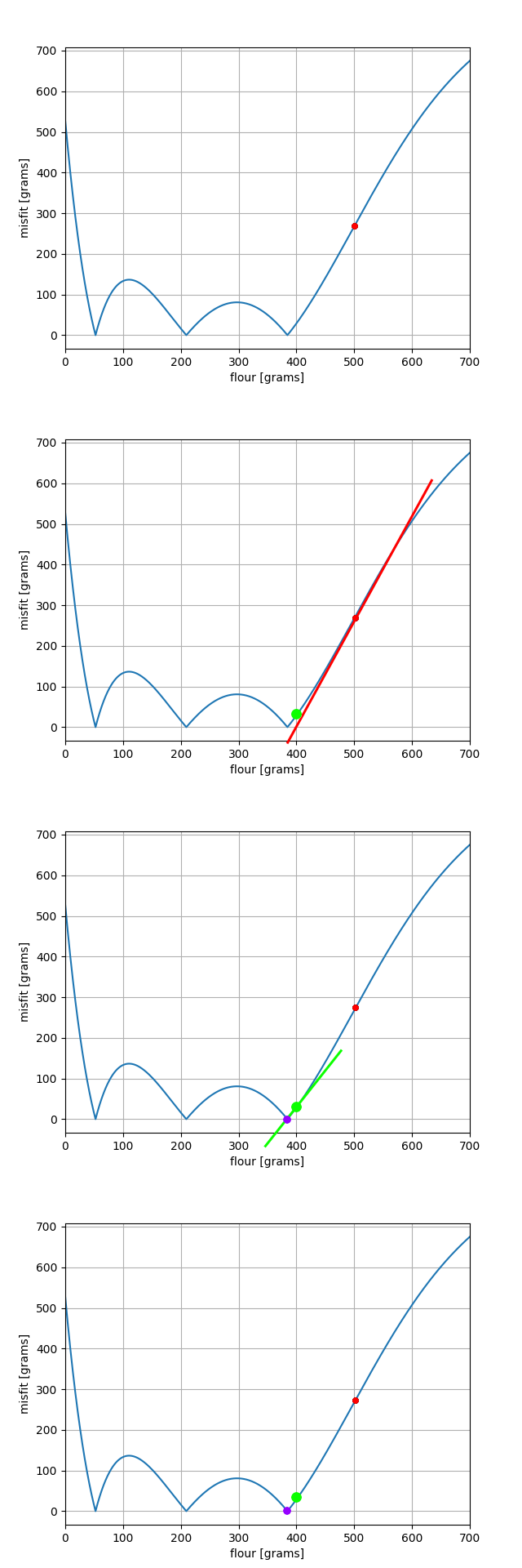
Simplistic gradient descent
Obvious solutions, grid searches, and higher dimensions
One thing that often bugged me about the aforementioned gradient descent methods is the seemingly complicated approach for such simple problems. Anyone looking at the figures could have said
Well, duh, there’s 3 solutions, here, here and here!
Why care about such an complicated way to only get one of them?
The important realisation to make here is that I have precomputed all possible solution for this forward model in the 0 – 700 grams range. This precomputation on a 1D domain was very simple; at a regular interval, compute the predicted value of baked bread. Following this, I could have also programmed my Python routine to extract all the values with a sufficiently low misfit as solutions. This is the basis of a grid search.
Let’s perform a grid search on our second model (1b). Let’s find all predictions with 500 grams of bread as the end result, plus-minus 50 grams. This is the result:
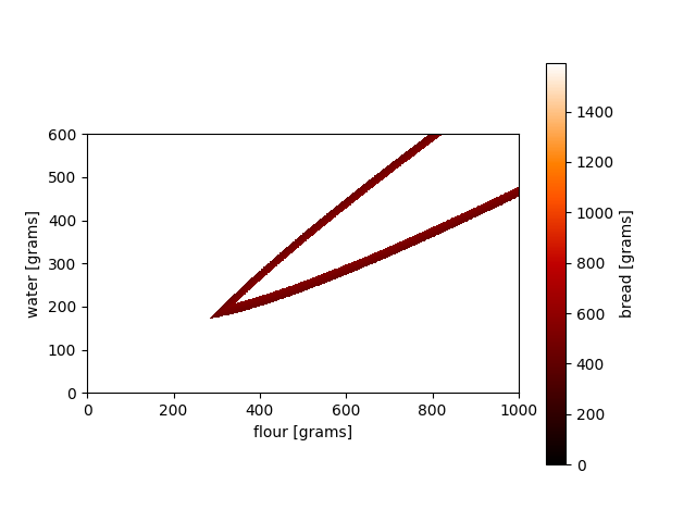
Grid search for the 2D model
The original 312.5 grams of flour as input is part of the solution set. However, the model actually has infinitely many solutions (extending beyond the range of the current grid search)! The reason that a grid search might not be effective is the inherent computational burden. When the forward model is sufficiently expensive in numerical simulation, exploring a model space completely with adequate resolution might take very long. This burden increases with model dimension; if more model parameters are present, the relevant model space to irrelevant model space becomes very small. This is known as the curse of dimensionality (very well explained in Tarantola’s textbook).
Another reason one might want to avoid grid searches is our inability to appropriately process the results. Performing a 5 dimensional or higher grid searches is sometimes possible on computational clusters, but visualizing and interpreting the resulting data is very hard for humans. This is partly why many supercomputing centers have in-house departments for data visualisation, as it is a very involved task to visualise complex data well.
Now: towards solving our physical inversions!
Non-uniqueness, regularization and linear algebra (bleh!)
One big problem in inversion is non-uniqueness: the same result can be obtained from different inputs. The go-to way to combat this is to add extra information of any form to the forward problem. In our bread recipe we could think of adding extra observables to our problem, such as the consistency of the bread, its taste, color, etc. Another option could be to add constraints on the parameters, such as using the minimum amount of ingredients. This is akin to asking the question: given this amount of bread, how much flour and water was minimally used to make it?
Diffusion type problems are notorious for their non-uniqueness. Many different subsurface heat conduction distributions might result in the observations (imagine differently inclined volcanic conduits). An often used method of regularisation (not limited to diffusion type studies!) is spatial smoothing. This method requires that among equally likely solutions, the smoothest solutions are favoured, for it is more ‘natural’ to have smoothly varying parameters. Of course, in many geoscientific settings one would definitely expect sharp contrasts. However, in ‘underdetermined’ problems (i.e., you do not have enough observations to constrain a unique solution), we favour Occam’s Razor and say
The simplest solution must be assumed
When dealing with more parameters than observables (non-uniqueness) in linear models it is interesting to regard the forward problem again. If one would parameterize our volcanic model using 9 parameters for the subsurface and combine that with the 3 measurements at the surface, the result would be an underdetermined inverse problem.

Rough parametrization for the heat conduction model
This forward model (the Laplace equation) can be discretised by using, for example, finite differences. The resulting matrix equation would be Am = d, with A a 3 x 9 matrix, m a 9 dimensional vector and d a 3 dimensional vector. As one might recall from linear algebra classes, for a matrix to have an inverse, it has to be square. This matrix system is not square, and therefore not invertible!
Aaaaahhh! But don’t panic: there is a solution
By adding either prior information on the parameters, smoothing, or extra datapoints (e.g., taking extra measurements in wells) we can make the 3 x 9 system a perfect 9 x 9 system. By doing this, we condition our system such that it is invertible. However, many times we end up overdetermining our system which could result in a 20 x 9 system, for example. Note that although neither the underdetermined nor the overdetermined systems have an exact matrix inverse, both do have pseudo-inverses. For underdetermined systems, I have not found these to be particularly helpful (but some geophysicists do consider them). Overdetermined matrix systems on the other hand have a very interesting pseudo-inverse: the least squares solution. Finding the least squares solution in linear problems is the same as minimising the L2 norm! Here, two views on inversion come together: solving a specific matrix equation is the same as minimising some objective functional (at least in the linear case). Other concepts from linear algebra play important roles in linear and weakly non-linear inversions. For example, matrix decompositions offer information on how a system is probed with available data, and may provide insights on experimental geophysical survey design to optimise coverage (see “Theory of Model-Based Geophysical Survey and Experimental Design Part A – Linear Problems” by Andrew Curtis).
I would say it is common practice for many geophysicists to pose an inverse problem that is typically underdetermined, and keep adding regularization until the problem is solvable in terms of matrix inversions. I do not necessarily advocate such an approach, but it has its advantages towards more agnostic approaches, as we will see in the post on probabilistic inversion next week!
Summary of deterministic inversions
We’ve seen how the forward model determines our inversion problem, and how many measurements can be combined into a single measure of fit (the misfit). Up to now, three inversion strategies have been introduced:
• Direct inversion: analytically find a solution to the forward problem. This method is limited to very specific simple cases, but of course yields near perfect results.
• Gradient descent methods: a very widely used class of algorithms that iteratively update solutions based on derivatives of the misfit function. Their drawbacks are mostly getting stuck in local minima, and medium computational cost.
• Grid searches: a method that searches the entire parameter space systematically. Although they can map all the features of the inverse problem (by design), they are often much too computationally expensive.
What might be even more important, is that we have seen how to reduce the amount of possible solutions from infinitely many to at least a tractable amount using regularisation. There is only one fundamental piece still missing… Stay tuned for the last blog post in this series for the reveal of this mysterious missing ingredient!
Interested in playing around with inversion yourself? You can find a toy code about baking bread here.