Introduction
Despite advances in our understanding of rock mechanics, the frictional behavior of rocks, and the physics of instability in geological materials, the coexistence of slow and fast earthquakes, as well as various types of fault-zone seismic radiation such as tremor, remains enigmatic.
Can fault mechanics and friction laws reproduce the full spectrum of observed seismicity?
In this week’s blog post, Navid Kheirdast takes us through the fundamentals of fault mechanics and frictional behavior before introducing a simple yet powerful mechanical model composed of a main fault interacting with a population of off-fault fractures. Despite its simplicity, the model captures a remarkable range of behaviors observed in nature, reproducing the spectrum of fault slip from slow slip events to fast, dynamic earthquakes.
1. Faults and the Forces They Bear
Faults are interfaces in Earth’s crust—boundaries between tectonic plates or between blocks within a plate—that are permanently subjected to background stress driven by plate tectonics and environmental loading (tides, fluid pressure, and so on). In response to this stress, the two sides of a fault slide past each other: this sliding motion is called slip.
To describe fault slip mechanically, we need two families of variables:
- Dynamic variables — the traction (force per unit area) acting on the fault surface, including frictional resistance and pore-fluid pressure.
- Kinematic variables — the relative displacement (slip) and slip rate across the fault.
The fault-slip problem is a boundary-value problem: knowing one set of variables (say, the background stress) allows us to solve for the other (slip rate). The relationship between stress and slip is governed by a friction law.
2. The Wide Spectrum of Fault Slip
Slip on natural faults spans an enormous range of speeds, from a few millimeters per year all the way to several meters per second. Three end-member behaviors stand out.
Creep
Creep is aseismic, quasi-static sliding at roughly the tectonic loading rate — that is, the fault slides continuously at the same speed that the two tectonic plates move relative to each other. No earthquakes occur on creeping faults. Famous examples include the Parkfield segment of the San Andreas Fault and parts of the North Anatolian Fault near the Sea of Marmara.
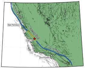
Creep across the San Andreas Fault. Credit: Coffey et al. (2022).
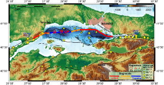
Creep across the North Anatolian Fault. Credit: Becker et al. (2023).
Slow Earthquakes
Sometimes slip is faster than the tectonic loading rate but far too slow to radiate significant seismic waves in the classical seismic stations, and only very accurate GNSS stations can record them. Such events — slow earthquakes (also called slow-slip events or SSEs) — may unfold over weeks to months rather than seconds. They are commonly observed in subduction zones: Cascadia, Nankai, Mexico, and Chile all host periodic slow-slip events.
Regular (Fast) Earthquakes
At the other extreme, slip accelerates to meters per second in a matter of seconds, releasing energy as the seismic waves we feel as earthquakes.
The central question is: what controls which of these behaviors a given fault segment will exhibit?
3. Fault Stability
There exists a critical stiffness for any fault segment under tectonic loading. If the fault is “stiff enough,” any small perturbation in slip rate dies out—the fault creeps stably. If the fault stiffness is below the critical value, perturbations grow, and an earthquake results.
Computing this instability threshold is an eigenvalue problem: the critical eigenvalue depends on the frictional properties of the fault surface. This insight was established experimentally by Brace & Byerlee (1966), who showed through triaxial rock-mechanics tests that laboratory rock samples under confining pressure produce stick-slip cycles — the laboratory analogue of repeated earthquakes.
4. Two Friction Laws for Fault Mechanics
Two friction laws dominate earthquake modeling, each capturing a different aspect of fault behavior.
4.1 Linear Slip-Weakening Friction
The simplest physically motivated friction law expresses resistance as a function of cumulative slip alone:
- At the onset of slip, friction equals the static strength τs = μsσ.
- As slip accumulates, resistance decreases linearly until it reaches a dynamic (residual) strength τd = μdσ after a characteristic slip distance Dc.
- Beyond Dc, friction stays constant at τd.
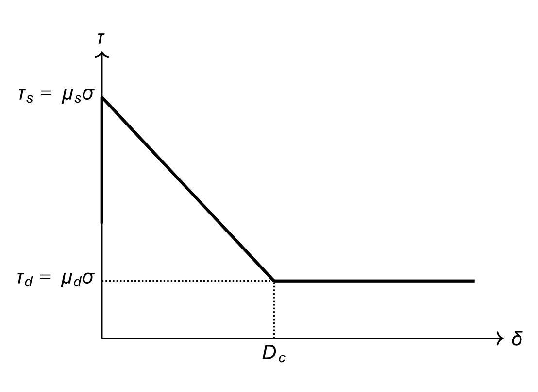
Slip-weakening diagram: τ vs. δ (slip), showing peak τs, linear weakening to τd over Dc, then flat residual.
Limitations of the slip-weakening law:
- No mechanism for friction recovery, or healing — once the fault has slipped past Dc, it cannot restore its previous strength.
- No rate dependence — friction does not depend on how fast the fault is sliding. This means that on a fault at the brink of instability, any infinitesimal increase in slip rate immediately triggers an earthquake, with no intermediate regime. Laboratory experiments, however, show that real surfaces resist sudden speed changes — they do not break instantly.
4.2 Rate-and-State Friction
Rate-and-state friction (RSF), formulated by Dieterich (1979) and Ruina (1983) on the basis of laboratory experiments, addresses both limitations. It expresses the friction coefficient as a function of slip rate v and a state variable φ:
μ = f* + a ln(v/v*) + b ln(θ/θ*)
where a is a constant related to the direct strength increase due to a jump in velocity, v* is a reference slip rate, and θ encodes the history of contact. The state variable evolves with slip and time, providing the fault with memory.
Two evolution equations for θ are widely used:
- Aging law — state evolves both with slip and with time (contacts strengthen even when stationary).
- Slip law — state evolves only when slip occurs; no healing without motion.
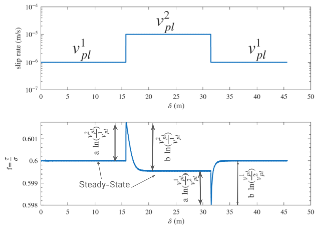
Velocity-step experiment: the top panel shows slip rate jumping from v1 to v2; the bottom panel shows the immediate increase in the friction coefficient μ, followed by gradual relaxation to the new steady-state value μss.
Key insight from RSF: If you suddenly increase the slip rate, friction immediately increases (the “direct effect”), but then slowly decreases back to a new steady-state value as θ evolves. The long-term (steady-state) friction level at speed v is:
τss(v) = μss(v) · σ, where Δμss = (a−b) ln(v2/v1)
- If a − b < 0: steady-state friction decreases with increasing slip rate → velocity-weakening behavior → potentially unstable.
- If a − b > 0: steady-state friction increases with increasing slip rate → velocity-strengthening behavior → inherently stable.
Limitation of RSF: It was calibrated in laboratory experiments at low slip rates (micrometers to millimeters per second), far below the meters-per-second speeds reached during large earthquakes. At coseismic rates, slip-weakening is thought to take over.
5. The Spring-Slider System — A Minimal Earthquake Cycle Model
The Burridge-Knopoff spring-slider is the simplest mechanical system that reproduces stick-slip cycles. A block rests on a frictional surface and is connected by a spring to a loading point that moves at a constant velocity vpl, representing the far-field tectonic loading rate.
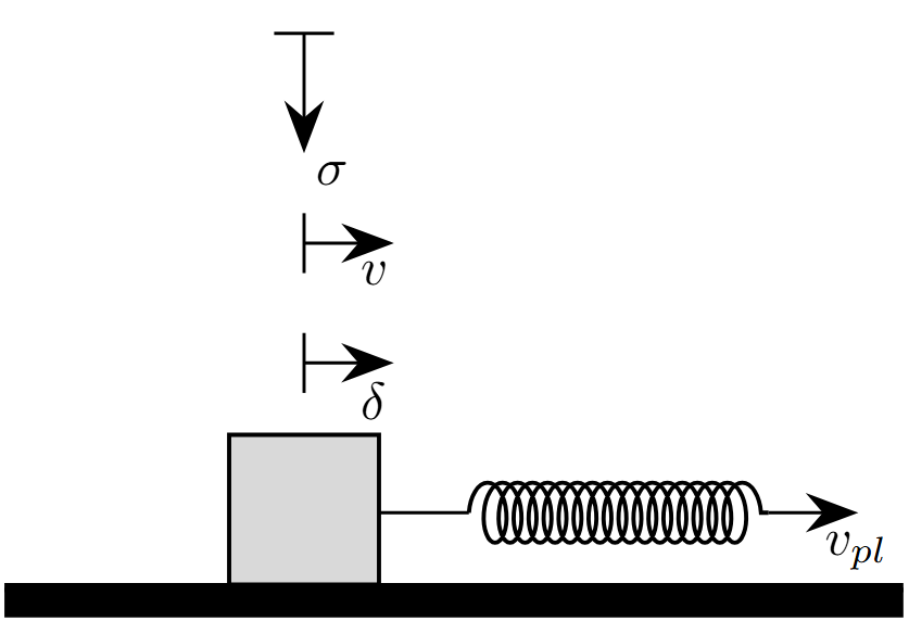
Spring-slider diagram: block on frictional surface, spring of stiffness k, loading point moving at v_pl; arrows showing slip δ, slip rate v, normal stress σ.
Two outcomes are possible:
- Stable sliding (creep): If the spring is stiff enough, the block slides at exactly vpl, smoothly and continuously.
- Stick-slip (earthquake cycles): If the spring stiffness falls below a critical value kc, the block sticks while the spring stretches, then suddenly lurches forward when the spring force exceeds static friction — mimicking an earthquake.
6. Critical Stiffness — Why Each Behavior Occurs
Linear Stability Analysis
To find the threshold between stable and unstable slip, Ruina (1983) performed a quasi-static linear stability analysis around the steady-state sliding solution of a slider on a rate and state surface. The method is to perturb the slip rate slightly away from steady state and ask whether the perturbation grows or decays. Details of this analysis is well explained by Segall (2010), therefore we recommend the interested reader to follow from the text book.
The critical stiffness gives:
kc = σ(b − a) / Dc
Physical Interpretation
The critical stiffness kc has a transparent physical meaning:
| Parameter | Role |
|---|---|
| σ | Normal stress — higher confining stress makes slip harder to control |
| b − a | Net velocity-weakening tendency — larger means more destabilizing |
| Dc | Characteristic slip distance — larger Dc means the fault “forgets” its history more slowly, which is stabilizing |
The Two Regimes at a Glance
| Condition | Behavior | Geological analog |
|---|---|---|
| k > kc (stiff) | Stable sliding | Aseismic creep |
| k < kc (compliant) | Stick-slip | Earthquake cycles |
7. Numerical Example — Pseudo-Dynamic Simulation
To see both regimes in action, we solve the spring-slider equations numerically, including a radiation-damping term ηv that approximates elastic wave effects without a full dynamic calculation:
σ(f* + a ln(v/v*) + b ln(v*θ/Dc)) = k(vplt − δ) − ηv
with the aging law θ̇ = 1 − vθ/Dc.
With parameters chosen so that a/b = 0.9 (velocity-weakening) and k/kc = 0.95 (the spring is just below the critical stiffness), the simulation produces periodic stick-slip cycles:
Increasing the spring stiffness slightly so that k/kc > 1 immediately switches the system to stable sliding:
These two simulations illustrate the core message: the same friction law and the same fault, but a single parameter crossing a threshold, separate creeping from seismogenic behavior.
8. Lack of Key Observations
The spring-slider model, which resembles a single fault, captures key features of seismic cycles, such as stick-slip and creep-like fault behavior, interseismic and coseismic phases, and periodic ruptures, but it misses some important features, such as the Gutenberg–Richter magnitude-frequency relation, the coexistence of slow and fast ruptures, aftershock sequences, and the localization of seismic activity. In a recent paper by Almakari, Kheirdast et al. (2026), the authors showed that considering the size distribution of off-fault fractures around a main fault produces all of these features.
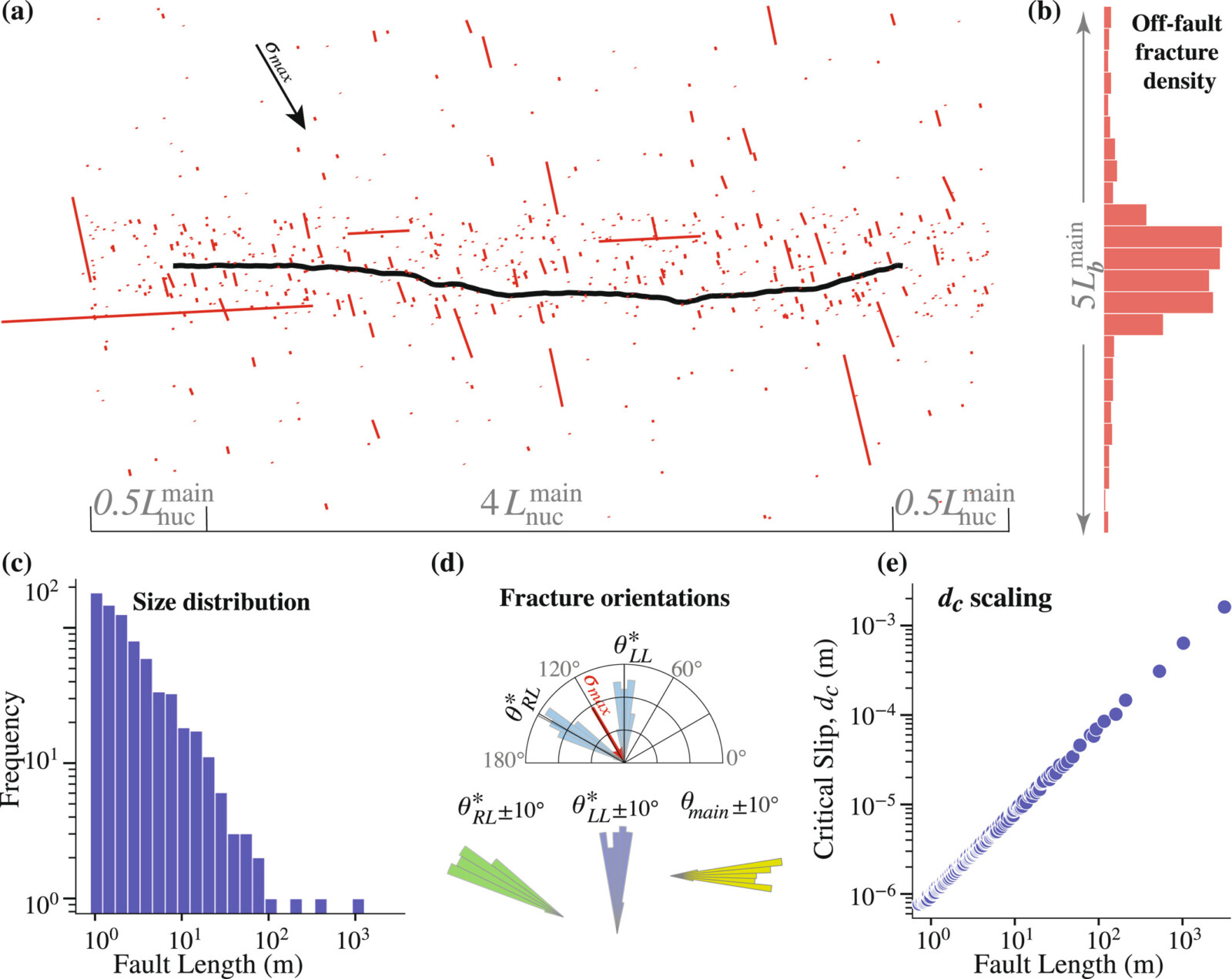
The fault-volume model as presented in Almakari et al. (2026). In this model, a main rough fault is embedded in a fault volume. Close to the main fault, there is a higher density of off-fault fractures; fracture density decreases with distance from the fault. The size distribution of off-fault fractures follows a power law. Off-fault fractures are oriented optimally with respect to the background stress loading, and all faults are strengthened by rate-and-state friction, with Dc scaling with fault length.
The results of this model interestingly reproduce all statistical properties observed in real catalogs, including the Omori and inverse Omori laws, the Gutenberg–Richter law, and scaling of fast ruptures as M ∼ T³ and slow events as M ∼ T.
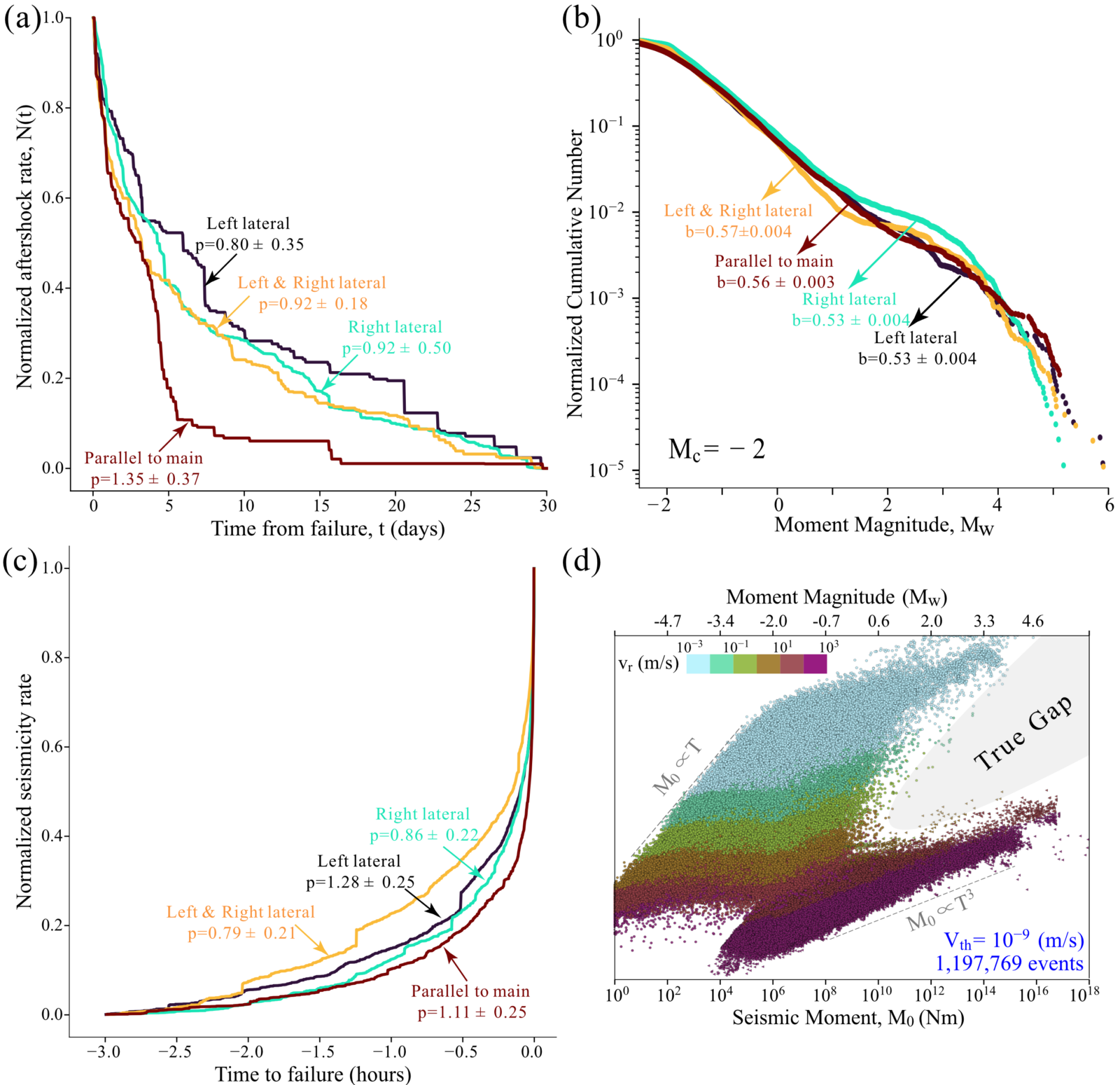
Statistics of fault-volume seismicity from Almakari et al. (2026): (a) Omori-law decay in seismic activity after mainshocks, (b) Gutenberg–Richter magnitude-frequency distribution, (c) inverse-Omori increase in seismic activity prior to the main rupture, and (d) scaling of the magnitude and distribution of events produced in the fault zone lies between the M ∼ T³ and M ∼ T limits.
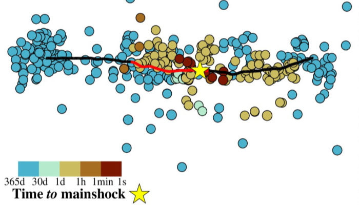
An intriguing result of the fault-volume model is the migration of events in the fault zone as time approaches the main shock; after the main shock, events tend to return to background seismicity:
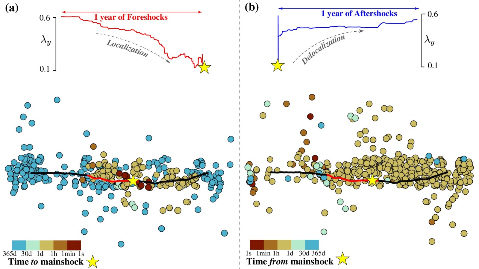
Migration of seismicity: (a) prior to the main shock, off-fault events tend to migrate toward the future event’s epicenter. (b) After the main rupture, activity returns to the fault volume, a process called delocalization (Ben-Zion and Zaliapin, 2020).
9. Conclusion
Fault slip is one of the most unpredictable processes in nature. Yet, as this post has shown, much of its complexity can be traced back to a surprisingly compact set of mechanical ingredients.
The wide spectrum of observed fault behaviors — from quiet aseismic creep, through slow-slip events that unfold over months, to sudden earthquake ruptures — is not the result of fundamentally different physical processes. It emerges from the interplay between frictional properties and the elastic stiffness of the surrounding crust. Rate-and-state friction, calibrated from laboratory rock experiments, captures the two key ingredients: a fault’s immediate resistance to speed changes (the direct effect) and its gradual loss or recovery of strength over time (the evolving state variable). When these are combined with a simple spring-slider geometry, a single dimensionless ratio — k/kc — determines whether the fault creeps or earthquakes.
Yet the single-fault spring-slider model, elegant as it is, cannot explain the full texture of real seismicity: the statistical distribution of earthquake sizes, the complex migration of activity in space and time, the coexistence of slow and fast events on the same fault system. The fault-volume model of Almakari, Kheirdast et al. (2026) demonstrates that bringing in off-fault fractures with a power-law size distribution — each obeying the same rate-and-state friction, each interacting mechanically with the main fault — is sufficient to recover all of these features at once. The Gutenberg–Richter law, Omori-law aftershock decay, inverse-Omori foreshock acceleration, and the characteristic scaling differences between slow and fast ruptures all emerge naturally from a single, self-consistent mechanical framework.
The broader lesson is one of emergent complexity from simple rules: a friction law grounded in laboratory physics, applied consistently across a geometrically realistic fault zone, reproduces phenomena that have long resisted explanation. This suggests that the enigmatic coexistence of slow and fast earthquakes, and the apparently erratic migration of seismic activity, may not require exotic physics — only a more complete account of the fault’s mechanical environment.
Understanding these mechanics has direct implications for seismic hazard assessment. If slow-slip events and tremors are governed by the same friction physics as regular earthquakes, they are not merely curiosities – they are windows into the stress state of fault zones, and potentially precursors to larger events. The migration patterns revealed by the fault-volume model, in particular, may one day inform operational monitoring strategies.
Much remains to be done. Validating model statistics against dense seismic catalogs are all open challenges. But the foundation laid by decades of friction experiments, stability theory, and increasingly realistic mechanical models gives good reason for optimism that a unified physical picture of fault-zone seismicity is within reach.
References

Almakari, M., Kheirdast, N., Villafuerte, C., Thomas, M. Y., Dubernet, P., Cheng, J., ... & Bhat, H. S. (2026). Fault volume digital twin to reproduce the full slip spectrum, scaling, and statistical laws. Journal of Geophysical Research: Solid Earth, 131(5), e2025JB032915.

Coffey, G. L., Savage, H. M., Polissar, P. J., Cox, S. E., Hemming, S. R., Winckler, G., & Bradbury, K. K. (2022). History of earthquakes along the creeping section of the San Andreas Fault, California, USA. Geology, 50(4), 516–521.

Becker, D., Martínez-Garzón, P., Wollin, C., Kılıç, T., & Bohnhoff, M. (2023). Variation of fault creep along the overdue Istanbul–Marmara seismic gap in NW Türkiye. Geophysical Research Letters, 50. [doi.org](https://doi.org/10.1029/2022GL101471)

Zhang, H., & Li, F. (2024). A review of prediction methods for global buckling critical loads of pultruded FRP struts. Composite Structures, 329, 117752. [doi.org](https://doi.org/10.1016/j.compstruct.2023.117752)

Brace, W. F., & Byerlee, J. D. (1966). Stick-slip as a mechanism for earthquakes. Science, 153(3739), 990–992.

Dieterich, J. H. (1979). Modeling of rock friction: 1. Experimental results and constitutive equations. Journal of Geophysical Research: Solid Earth, 84(B5), 2161–2168.

Ruina, A. (1983). Slip instability and state variable friction laws. Journal of Geophysical Research: Solid Earth, 88(B12), 10,359–10,370.

Rice, J. R. (1993). Spatio-temporal complexity of slip on a fault. Journal of Geophysical Research: Solid Earth, 98(B6), 9885–9907.

Cochard, A., & Madariaga, R. (1994). Dynamic faulting under rate-dependent friction. Pure and Applied Geophysics, 142(3–4), 419–445.

Ben-Zion, Y., & Zaliapin, I. (2020). Localization and coalescence of seismicity before large earthquakes. Geophysical Journal International, 223(1), 561–583.

Segall, P. (2010). Earthquake and volcano deformation.