Computational geodynamic models are powerful tools for understanding Earth’s deep interior, but how do we know they are producing realistic results? In this week’s News & Views, Alina Valop, a PhD candidate from Virginia Tech, unpacks the world of geodynamic kernels and shows how these sensitivity functions provide a computationally efficient way to benchmark mantle flow models, test viscosity structures, and bridge the gap between numerical simulations and geophysical observations.

Alina Valop from Virginia Tech
“You should produce the kernels and compare them to the benchmark paper,” said my advisor. Perfect, I shall do that. And the first step is to find out what kernels are. Surely the internet will have a straightforward answer…
And it did: the internet gave me kernel definitions for operating systems, statistics, and popcorn, just not geodynamic kernels. But I still needed to know whether my model was behaving correctly. Based on the literature, it came down to this: for a benchmark in a 3D mantle model, a kernel shows how the model responds when I place a density anomaly at one depth; repeating this at every depth produces a curve (Green’s function) that I could compare with a published curve. If they matched, I knew that part of my model was behaving correctly. Easy peasy, we can move on! Except we cannot, because while looking into who was using kernels and why, my advisor suggested I read Hager and Clayton (1989) to understand how kernels can be used for more than just benchmarking.
Let’s state some facts:
- 3D geodynamic models are computationally expensive.
- There’s a multitude of possible viscosity models we can assign to the mantle.
- And all the while, seismic tomography has considerably more detailed and reliable data than we’ve ever had (shoutout to the EarthScope stations).
- Different models often disagree in amplitude and smaller features. When you have enough parameters to adjust, you can make almost anything fit. As a professor once said, “Tell me how many cats you want to fit in your model, and we’ll make it happen.”
If only there were a computationally inexpensive way to test these models, compare them to the data we have, and narrow them to a realistic number of possibilities to commit to a 3D calculation… Spoiler alert: that’s kernels!
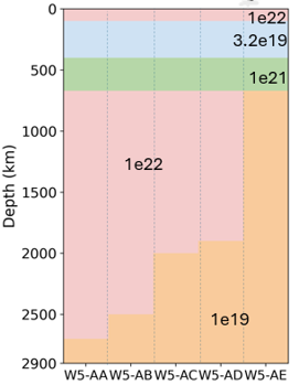
Figure 1. Five radial viscosity profiles used in the thickness experiment (W5-AA through W5-AE). Each color is one viscosity layer. The viscosity values stay fixed, while the weak 10¹⁹ Pa s layer above the CMB thickens from 200 km in AA to 2230 km in AE. Depth increases downward.
What are kernels?
Kernels are sensitivity functions for theoretical density anomalies. For example, in a 1D model of the Earth with a density and viscosity assigned at each depth (Figure 1), you can systematically test how sensitive a boundary (the geoid, surface topography, or core-mantle boundary (CMB) topography) is to an anomaly at each depth. To do this, we solve the Stokes equations in a spherical shell and calculate the radial response function Kl(r) for each spherical harmonic degree. The degree tells us the horizontal size of the pattern at the boundary. Degree 2 describes the largest wavelength pattern, which is the focus of this example, while higher degrees describe smaller-scale patterns. When the value of Kl(r) is positive, a positive density anomaly at that depth contributes positively to the boundary. When it is negative, the anomaly contributes to the opposite direction.
But conceptually it gets simpler: for the boundary ΔBlm you want to identify (geoid, surface topography or CMB topography), you multiply the kernel value Kl(r) by the density anomaly δρlm(r) at each depth, then add the contributions from the CMB to the surface. The result (ΔBlm) is a spherical harmonic coefficient for the geoid, surface topography, or CMB topography, depending on which kernel you calculate. In other words, the kernel tells you, “If you have a density anomaly at r depth, under your current model conditions, it will affect your boundary by this much (Figure 2).”
Here is the best part: if you change your radial viscosity, the kernel response changes (Figure 3). For this experiment, you keep the density model fixed and compute a new kernel, which means you can test multiple viscosity ideas while changing only one or two parameters at a time. Density still affects the final amplitude; keeping it fixed here simply lets us see what viscosity is doing.
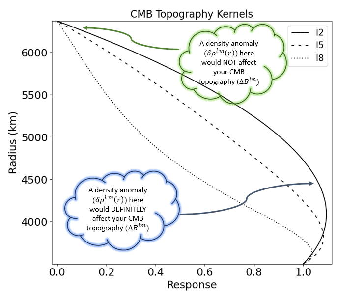
Figure 2. Core-mantle boundary topography kernels for a uniform-viscosity, uniform-density model. Each line shows the response to a different spherical harmonic degree. The y-axis represents radius, and the x-axis represents relative response.
Case study: the lower mantle needs some zest
To explain their capability, we need to consider what we want to predict. In my case, it is CMB topography. The CMB separates the solid mantle and the liquid core at ~2900 km dept and topography estimates find it to be roughly 300-4000 m (Deschamps et al., 2018; Heyn et al., 2020; Koelemeijer, 2021). However, there is no consensus on the direction, exact pattern, or amplitude of topography produced by mantle flow, only in the location of topography beneath the African and Pacific Large Low Shear Velocity Provinces (LLSVPs; Koelemeijer, 2021; Lekic et al., 2012). All this to say, CMB topography is a very useful constraint, but not a perfect answer.
In this case, a kernel tells us how efficiently a density anomaly at any depth would be transmitted to the CMB (Figure 3). As the kernel shows, anomalies near the surface have negligible weight on our CMB topography observation. The density anomalies come from a geodynamicist’s close friend, aka tomography. For this example, we will use SP12RTS (Figure 3; Koelemeijer et al., 2016) and focus on degree 2, the largest-scale structure in the lower mantle and CMB.
Tomography measures seismic velocity, not density, so we convert the anomalies using mineral physics (Figure 3 – CMinPhys). In this example, we use a uniform factor of 0.25 across the range discussed by Adam et al. (2021). If only this factor changes, the predicted topography changes linearly. Density, therefore, matters for amplitude; keeping it fixed isolates the effect of viscosity.
This is where Hager and Clayton’s model 5 (W5 and blue line in the kernel Figure 3) returns to the story. W5 has a relatively strong 10²² Pa s lower mantle and a weaker 10¹⁹ Pa s layer directly above the CMB. A weak D″ layer can reduce the mechanical coupling between CMB topography and convection above it (Hager & Clayton, 1989). This inspires the question: if we hold the weak-layer viscosity fixed, how much does its thickness change the CMB response?
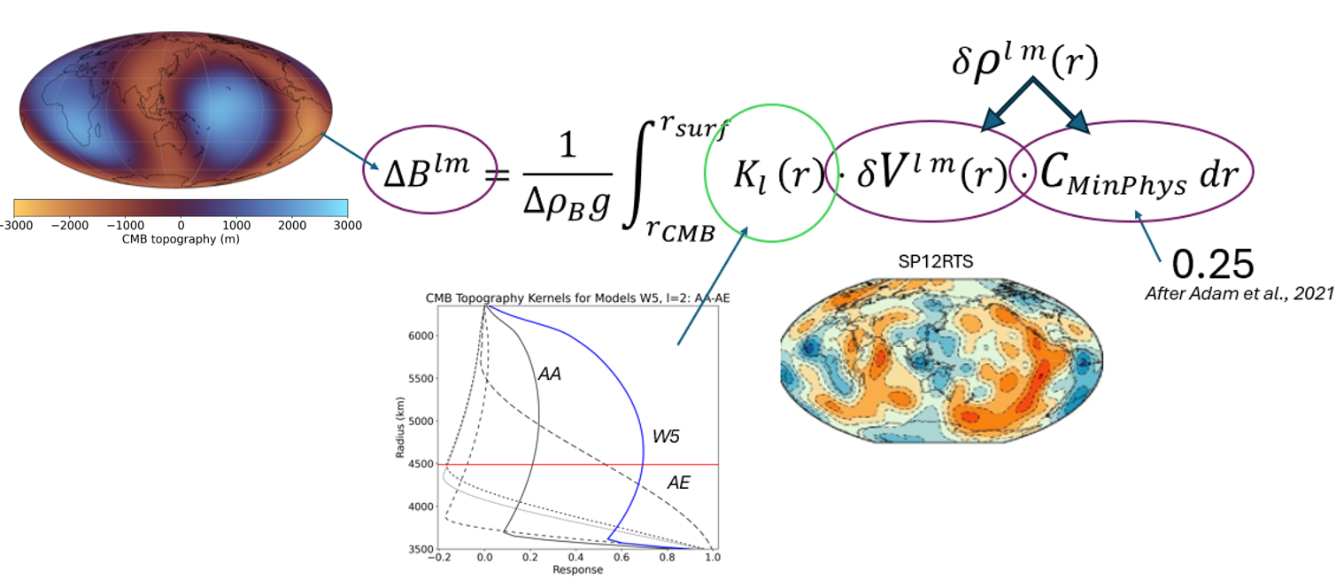
Figure 3. How the CMB topography (ΔB^lm) calculation comes together. The kernel (K_l (r) and respective figure) weights the SP12RTS tomography models at each depth (δρ^l m (r) and tomography slice). A factor of 0.25 converts velocity anomalies to density, and the contributions are added to predict CMB topography. The small graph compares the degree-2 kernels for the W5 models; radius increases from the CMB to the surface.
Models AA–AE test this question. We keep all viscosity values and the upper-mantle structure fixed; only the weak layer’s thickness changes: 200 km (AA), 400 km (AB), 900 km (AC), 1000 km (AD), and 2230 km (the whole lower mantle; AE). The result gives the maximum and minimum CMB topography calculated from SP12RTS, as shown in Table 1.
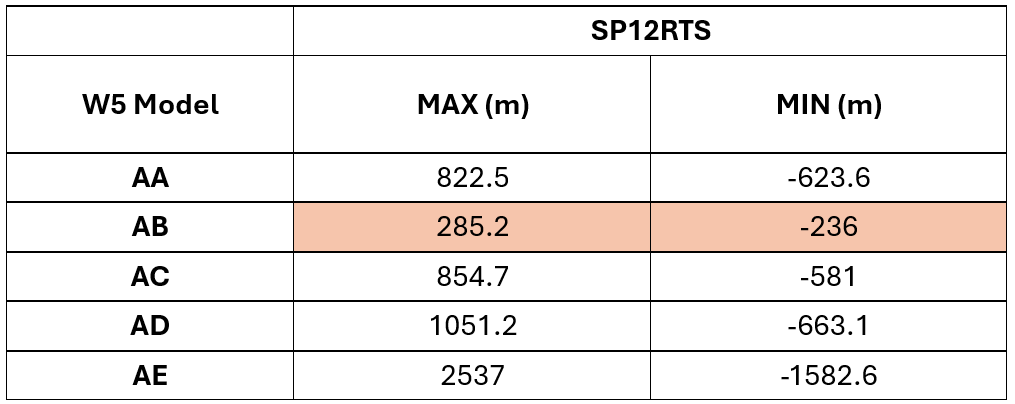
Table 1. Maximum and minimum degree-2 CMB topography predicted from SP12RTS for models AA–AE.
Almost every model in this suite produces topography within the broad range of 300–4000 m; AB falls just below it. The response is not steady as the weak layer thickens: AB is the smallest and AE the largest. And here is where you decide what still needs testing. Model AE, where the lower mantle is two orders of magnitude weaker than the transition zone, produces acceptable CMB topography, but that does not make it a realistic representation of the Earth. If we test that model in 3D (and I have), LLSVP-like piles cannot be maintained because the lower mantle is too weak. A profile also needs to satisfy the geoid or surface topography constraints, as it does the CMB topography. All this is to say that one boundary can shorten the list of possible models, but it cannot identify a unique Earth model by itself (Liu & Zhong, 2016; Steinberger & Calderwood, 2006). This work is part of a paper that explores other viscosity suites and compares different tomography models, currently in preparation for submission.
Don’t stop at the CMB!
Nothing about this workflow is limited to the CMB; that’s just what I like to study. The same calculation produces kernel responses for surface topography and the geoid in the current pipeline, following King and Masters (1992). These are (from a data availability standpoint) more attractive because Earth’s surface and gravity field are measured in far more detail than the CMB topography. The geoid has long been used to constrain radial mantle viscosity, including in tomography-driven flow models (Hager & Clayton, 1989; Liu & Zhong, 2016).
1D to 3D
As explained, kernels cannot identify “the one” viscosity profile, and a 1D model cannot represent laterally varying piles, slabs, plumes, or the lithosphere by itself. Instead, it allows us to shortlist the candidates we want to test in 3D, using realistic geometry and time evolution. 1D gives us a filter, and we let 3D handle the regional complexity.
So I am bringing kernels back to test Earth models fast. We have the best data anyone has ever had, and we should take advantage of it to go crazy with our tests. And if you’re ever asked about kernels, now you know why they’re cool, in with the old and the new!
References:

Adam, C., King, S. D., & Caddick, M. J. (2021). Mantle temperature and density anomalies: The influence of thermodynamic formulation, melt, and anelasticity. Physics of the Earth and Planetary Interiors, 319(September 2020), 106772. https://doi.org/10.1016/j.pepi.2021.106772

Deschamps, F., Rogister, Y., & Tackley, P. J. (2018). Constraints on core-mantle boundary topography from models of thermal and thermochemical convection. Geophysical Journal International, 212(1), 164–188. https://doi.org/10.1093/gji/ggx402

Hager, B. H., & Clayton, R. W. (1989). Constraints on the structure of mantle convection using seismic observations, flow models, and the geoid. In W. R. Peltier (Ed.), Mantle convection: Plate tectonics and global dynamics (pp. 657–763).

Heyn, B. H., Conrad, C. P., & Trønnes, R. G. (2020). Core-mantle boundary topography and its relation to the viscosity structure of the lowermost mantle. Earth and Planetary Science Letters, 543, 116358. https://doi.org/10.1016/j.epsl.2020.116358

King, S. D., & Masters, G. (1992). An Inversion For Radial Viscosity Structure Using Seismic Tomography. Geophysical Research Letters, 19(15), 1551–1554.

Koelemeijer, P. (2021). Towards consistent seismological models of the core–mantle boundary landscape. In Mantle convection and surface expressions (pp. 229–255). https://doi.org/10.1002/9781119528609.ch9

Koelemeijer, P., Ritsema, J., Deuss, A., & van Heijst, H. J. (2016). SP12RTS: A degree-12 model of shear- and compressional-wave velocity for Earth’s mantle. Geophysical Journal International, 204(2), 1024–1039. https://doi.org/10.1093/gji/ggv481

Lekic, V., Cottaar, S., Dziewonski, A., & Romanowicz, B. (2012). Cluster analysis of global lower mantle tomography: A new class of structure and implications for chemical heterogeneity. Earth and Planetary Science Letters, 357–358, 68–77. https://doi.org/10.1016/j.epsl.2012.09.014

Liu, X., & Zhong, S. (2016). Constraining mantle viscosity structure for a thermochemical mantle using the geoid observation. Geochemistry, Geophysics, Geosystems, 17(3), 895–913. https://doi.org/10.1002/2015GC006161

Steinberger, B., & Calderwood, A. R. (2006). Models of large-scale viscous flow in the Earth’s mantle with constraints from mineral physics and surface observations. Geophysical Journal International, 167(3), 1461–1481. https://doi.org/10.1111/j.1365-246X.2006.03131.x