Inverse theory exists to make the life of the mantle geodynamicist easier.
The Geodynamics 101 series serves to showcase the diversity of research topics and methods in the geodynamics community in an understandable manner. We welcome all researchers – PhD students to professors – to introduce their area of expertise in a lighthearted, entertaining manner and touch upon some of the outstanding questions and problems related to their fields. This time, Lars Gebraad, PhD student in seismology at ETH Zürich, Switzerland, talks about inversion and how it can be used in geodynamics! Due to the ambitious scope of this topic, we have a 3-part series on this with the next part scheduled for publication next week! This week, however, we start with the basics that many geodynamicists will be familiar with: the forward problem.
 Inversion methods are at the core of many physical sciences, especially geosciences. The term itself is used mostly by geophysicists, but the techniques employed can be found throughout investigative sciences. Inversion allows us to infer our surroundings, the physical world, from observations. This is especially helpful in geosciences, where one often relies on observations of physical phenomena to infer properties of the (deep) otherwise inaccessible subsurface. Luckily, we have many, many algorithms at our disposal! (…cue computer scientists rejoicing in the distance.)
Inverse theory in a nutshell
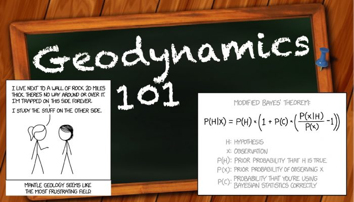
Credit: xkcd.
The process of moving between data and physical parameters goes by different names in different fields. In geophysics we mostly use inversion or inference. Inversion is intricately related to optimization in control theory and some branches of machine learning. In this small series of blog posts, I will try to shed a light on how these methods work, and how they can be used in geophysics and in particular geodynamics! In the end, I will focus a little on Bayesian inference, as it is an increasingly popular method in geophysics with growing potential. Be warned though:
Math ahead!
(although as little as possible)
First, for people who are serious about learning more about inverse theory, I strongly suggest Albert Tarantola’s “Inverse Problem Theory and Model Parameter Estimation”. You can buy it or download it (for free!) somewhere around here: http://www.ipgp.fr/~tarantola/.
I will discuss the following topics in this blog series (roughly in order of appearance):
1. Direct inversion
2. Gradient descent methods
3. Grid searches
4. Regularization
5. Bayesian inference
6. Markov chain Monte Carlo methods
The forward ‘problem’
Rather backwards, I will start the first blog post with a component of inversion which is needed about halfway through an inversion algorithm. However, this piece determines the physics we are trying to investigate. Choosing the forward ‘problem’ or model is posing the question of how a physical system will evolve, typically in a deterministic setting. This can be any relationship. The forward problem is roughly the same as asking:
I start with these materials and those initial conditions, what will happen in this system?
In this post I will consider two examples of forward problems (one of which is chosen because I have applied it everyday recently. Hint: it is not the second example…)
1. The baking of a bread with known quantities of water and flour, but the mass of the end product is unknown. A recipe is available which predicts how much bread will be produced (let’s say under all ratios of flour to water).
2. Heat conduction through a volcanic zone where geological and thermal properties and base heat influx are known, but surface temperatures are unknown. A partial differential equation is available which predicts the surface temperature (heat diffusion, Laplace’s equation).
Both these systems are forward problems, as we have all the necessary ingredients to simulate the real world. Making a prediction from these ‘input’ variables is a forward model run, a forward simulation or simply a forward solution. These simulations are almost exclusively deterministic in nature, meaning that no randomness is present. Simulations that start exactly the same, will always yield the same, predictable result.
Modelling our bread
For the first system, the recipe might indicate that 500 grams of flour produce 800 grams of bread (leaving aside the water for a moment, making case 1a), and that the relationship is linear in flour. The forward model becomes:
flour * 800 / 500 = bread
This is a plot of that relationship:
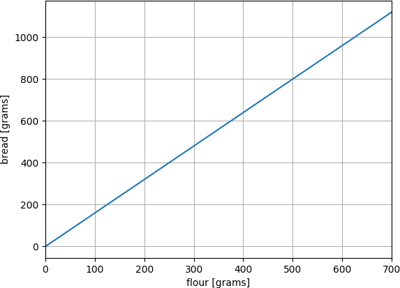
Simple flour to bread relationship: a 1D forward model.
I think I am getting hungry now. Does anyone else have the same problem?
Of course, if we add way too much water to our nice bread recipe, we mess it up! So, the correct amount of water is also important for making our bread. Hence, our bread is influenced by both quantities, and the forward model is a function of 2 variables:
bread = g(flour, water)
Let’s call this case 1b. This relationship is depicted here:

Simple flour and water to bread relationship: a 2D forward model.
Yes, I am definitely getting hungry.
It is important to note that the distinction between these two cases creates two different physical systems, in terms of invertibility.
Modelling our volcanic zone (and other PDE’s)
Modelling a specific physical system is a more complicated task. Typically, physical phenomena can be described by set of (partial) differential equations. Other components that are required to predict the end result of a physical deterministic system are
1. The domain extent, suitable discretisation and parameter distribution in the area of investigation, and the relevant material properties (sometimes parameters) at every location in the medium
2. The boundary conditions, and when the system is time varying (transient), additional initial conditions
3. A simulation method
As an example, the relevant property that determines heat conduction is the heat conductivity at every location in the medium. The parameters control much of how the physical system behaves. The boundary and initial conditions, together with the simulation methods are very important parts of our forward model, but are not the focus of this blog post. Typically, simulation methods are numerical methods (e.g., finite differences, finite elements, etc.). The performance and accuracy of the numerical approximations are very important to inversion, as we’ll see later.
The result of the simulation of the volcanic heat diffusion is the temperature field throughout the medium. We might however be only interested in the temperature at real-world measurement points. We consider the following conceptual model:
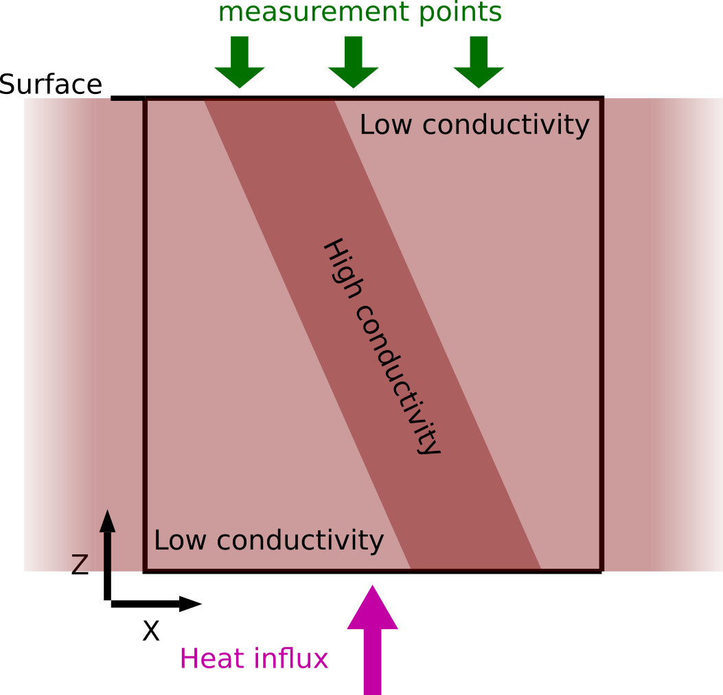
Conceptual model of heat diffusion in a heterogeneous thermal conductivity model. Domain of interest is the black box. Under homogeneous heat influx, the deterministic simulation will result in a decreasing temperature in the three measurement points from left to right.
The resulting temperatures at the measurement locations will be different for each point, because they are influenced by the heterogeneous subsurface. Real-world observations would for example look something like this
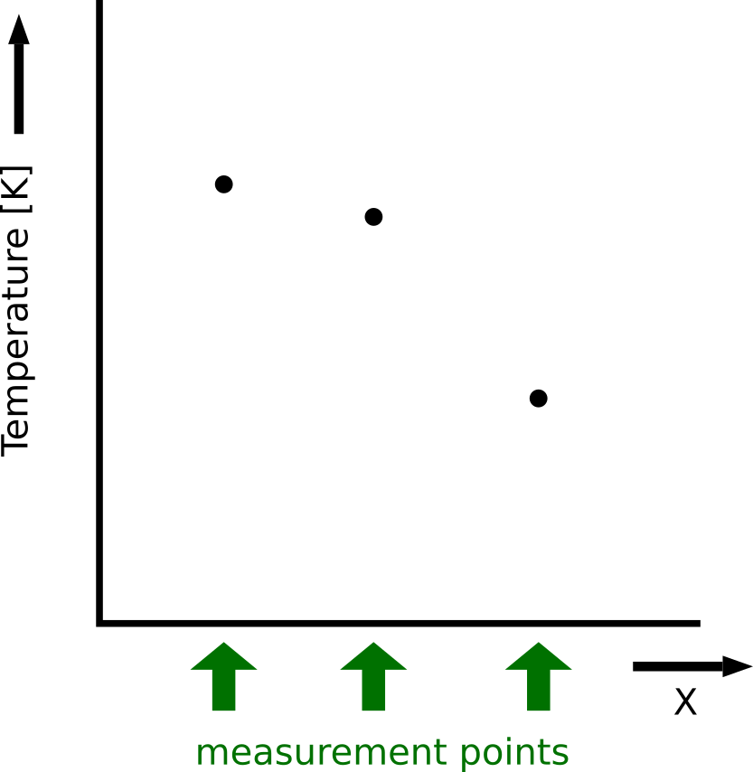
‘Observations’ (made by me of course) from the volcanic model.
Now that you have a good grasp of the essence of the forward problem, I will discuss the inverse problem in the next blog post. Of course, the idea of inversion is to literally invert the forward problem, but if it were as easy as that, I wouldn’t be spending 3 blog posts on it, now would I?