
Due to huge difference between the time scale of the mantle convection and the outer core convection, they are modelled separately. In this week’s News and Views, Masaki Yoshida from the Volcanoes and Earth’s Interior Research Center, Japan Agency for Marine-Earth Science and Technology (JAMSTEC), Japan, put forward the recent development on the modeling of the whole solid-Earth.

The Earth is composed of the rocky mantle and liquid core, which are considered to thermally and mechanically interact at their interface (i.e., core-mantle boundary; CMB) throughout the Earth’s history. The heat of the Earth’s interior has been slowly released to outer space at the Earth’s surface by not only the secular cooling of the Earth but also thermal convection in the mantle and the core. Thus, one of the major challenging issues in geodynamics is to numerically simulate thermal convection of these two layers in a unified thermal convection system, and resolve outstanding issues related to the dynamics of mantle-core interaction. However, previous numerical simulations of mantle convection and outer core convection have been performed independently by different researchers, different numerical codes, and different numerical techniques (Fig. 1). This is because the timescales of convection between the two layers differ vastly owing to the extremely large viscosity contrast between the rocky mantle and liquid core. Therefore, the simulation methods required to solve the basic equations of thermal convection are fundamentally different between mantle convection and outer core convection.
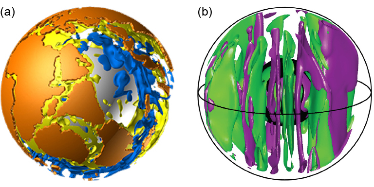
Figure 1. Examples of the 3D snapshots from numerical simulations of (a) mantle convection (Yoshida and Hamano, 2015) and (b) core convection with dynamo action (Aurnou et al., 2015).
Here, to aim for “Whole Solid-Earth Numerical Simulation,” we have started to develop a numerical simulation model of layered thermal convection with a large viscosity contrast based on a finite-volume method and numerical techniques used in mantle convection simulation. In order to give priority to a computational resolution over the real Earth 3D geometry, the computational model was confined in 2D spherical geometry with a highly viscous outer layer with a thickness of 2891 km (i.e., mantle) and a low-viscosity inner layer with a thickness of 3480 km (i.e., outer core) (Fig. 2a). The heat source that drives convection was simply assumed to be uniformly distributed in the whole convection domain. The key characteristic of our numerical model is that no artificial boundary condition was imposed at the CMB, and instead, a Gaussian-type function with a negative “effective thermal expansion coefficient” (e.g., Schubert et al., 1975) was imposed at the CMB, so that the two layers are fully continuously interacted each other. In this study, the mantle viscosity was fixed at a realistic value of 1021 Pa s, and the outer core viscosity was decreased from 1021 Pa s to the lower value. From our preliminary numerical tests treating the viscosity contrast between the mantle and the outer core as a free parameter, we found that the viscosity contrast between the two layers could be increased by up to three orders of magnitude (ΔηL ≤ 103) in the current supercomputational power and resource (Fig. 2b).
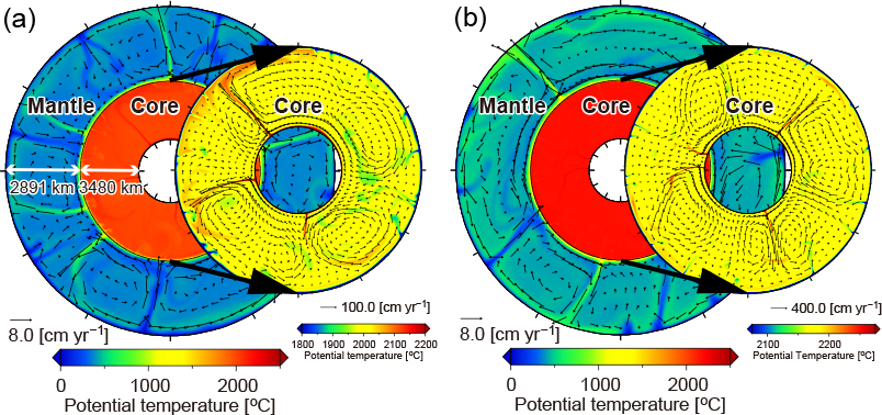
Figure 2. Snapshots of temperature and velocity fields in two-layered thermal convection (Yoshida et al., 2017). The mantle viscosity was fixed at 1021 Pa s, and the viscosity contrasts between the mantle and the outer core were set as (a) ΔηL = 101 and (b) ΔηL = 103.
Before understanding our numerical results quantitatively, we need to refer to fundamental dynamics in a two-layered thermal convection system with a viscosity contrast. In fluid dynamics, it is considered that there are two end-member coupling modes of two-layered convection, i.e., “mechanical (or viscous) coupling mode” (Fig. 3a) and “thermal coupling mode” (Fig. 3c) (e.g., Johnson and Narayanan, 1997; Yoshida and Hamano, 2016). The flow directions across the two layers are essentially inconsistent under the mechanical coupling mode (Fig. 3a), whereas, as increasing the viscosity contrast, the flow directions across the two layers tend to be consistent under the thermal coupling mode (Fig. 3c). Considering a huge viscosity contrast between the mantle and the outer core of the real Earth (ΔηL > 1020), the coupling mode would be classified into the thermal coupling mode. The “transitional mode” that we first proposed is an intermediate regime of these two modes (Fig. 3b), which is applicable to our model with ΔηL = 103 (Fig. 2b).
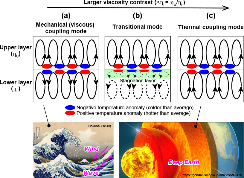
Figure 3. Coupling modes in two-layered thermal convection. The viscosity contrast between the two layers is ΔηL= ηu/ηL, where ηu and ηL are the viscosities of the upper and lower layers. The flow between the atmosphere (i.e., wind) and ocean (i.e., wave) is coupled under the mechanical (or viscous) coupling mode.
Our first numerical study of two-layered convection with a large viscosity contrast demonstrated that the behavior of mantle convection controls the convective style in the outer core and the heat transport efficiency of the whole solid-Earth (Yoshida and Hamano, 2016). Although the effective Rayleigh number of the outer core is increased (Fig. 4a) and the heat flow and the temperature at the CMB are increased as increasing ΔηL under the transitional mode (Fig. 4b), the flow speed and the heat transport efficiency of the mantle are close to being constant and temporally stabilized (see “P” and “Q” in Figs. 4c and d; in particular, the average mantle velocity goes to about 5cm/year for ΔηL = 102 and 103. This is because the convective flow in the highly viscous mantle drags the low-viscosity fluid in the topmost part of the outer core to make a “stagnation layer” (Fig. 3b). Our numerical result and theoretical estimation demonstrated that the transitional mode was observed when ΔηL was up to the order of approximately 102, and the switching between the mechanical and thermal coupling modes is initiated by the instability in the stagnation layer (Yoshida et al., 2017).
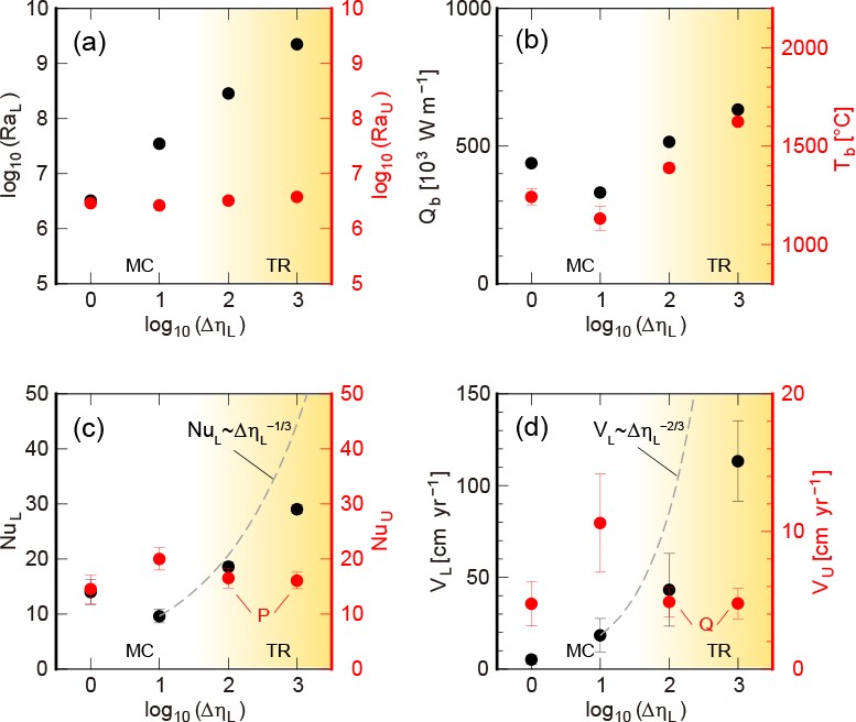
Figure 4. Analyses of the simulation result for each case with a different viscosity contrast between the two layers (ΔηL). (a, c, and d) ΔηL versus (a) the spatial-temporal averaged effective Rayleigh number, Ra (i.e., a measure of the vigor of convection), (c) the spatial-temporal averaged Nusselt number, Nu (i.e., a measure of heat transport efficiency), and (d) the spatial-temporal averaged (root-mean-square) flow speed, V, in the outer core (left vertical axis) and the mantle (right vertical axis). Note that in (a), (c) and (d), the black dots represented by the left axis are for the outer core and the red dots represented by the right axis are for the mantle. (b) ΔηL versus the averaged core-mantle boundary (CMB) heat flow, Qb (left vertical axis), and the temperature at the CMB, Tb (right vertical axis). MC and TR indicate the mechanical coupling and transitional modes. Modified from Yoshida and Hamano (2016).
From mineral physics experiments, it is considered that the inner core, which is composed of solidified iron, has started to grow in the Proterozoic era, although the exact birth age is still under debate (e.g., Dobson, 2016). In our subsequent study (Yoshida, 2018), we considered the growth of the inner core with a high viscous fluid, whose radius was just set as a function of age (Fig. 5). The result demonstrated that the average temperature of the outer core decreases significantly and the root-mean-square velocity of the outer core fluctuates significantly when the inner core grows with time (Fig. 5b), compared to the model without the growing inner core (Fig. 5a). The growth of the inner core enhances the vigor of core convection and the cooling of the outer core owing to the upwelling plumes originated from a boundary between the outer core and the growing inner core.
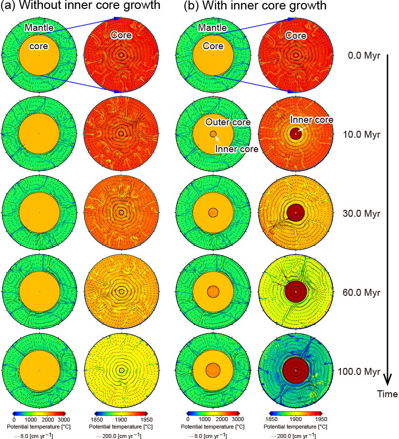
Figure 5. Temporal evolution of whole solid-earth convection (a) without and (b) with a growing inner core (Yoshida, 2018). The inner core was assumed to grow for 100 million years in this preliminary simulation.
One of the important results from a series of our preliminary “Whole Solid-Earth Numerical Simulation” is that the heat transport from the outer core to the mantle and the resultant flow speed of mantle convection is suppressed than we expected from a boundary-layer theory (Turcotte and Oxburgh, 1967; Olson and Corcos, 1980) in one-layer isoviscous convection, even though the outer core convection is very vigorous due to its low-viscosity (gray dashed lines in Figs. 4c and 4d). Thus, we suggested that in the real Earth, such a “stable” flow of mantle convection results in both “stable” plate tectonics and continental drift in a geological time scale and a very slow cooling of the Earth during its history (Fig. 6).
In the future, we need to further decrease the outer core viscosity with the advance of computational power and clarify the dynamics of the mantle-core interaction under the thermal coupling mode. Some previous geodynamo simulations demonstrated that the convection pattern in the outer core and the strength of the dipolar component of the geomagnetic field critically depend on the thermal and mechanical boundary conditions at the CMB (e.g., Dharmaraj et al., 2014). As implicitly suggested from a previous geodynamo simulation (Buffett, 2009), we proposed that the thermal and mechanical state in the topmost part of the outer core just beneath the CMB may be a clue to understanding generation mechanisms of the geomagnetic field (Yoshida, 2018; 2019), which plays an important role in protecting life on Earth from harmful solar winds in space.
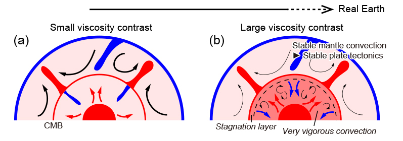
Figure 6. Cartoons showing the possible mantle-core interaction from our “Whole Solid-Earth Numerical Simulation.” (a) Case with a small viscosity contrast (ΔηL) between the mantle and the outer core under the mechanical coupling mode. (b) Case with a large ΔηL under the transitional or the thermal coupling modes.
References

Aurnou, J. M., Calkins, M. A., Cheng, J. S., Julien, K., King, E. M., Nieves, D., Soderlund, K. M. & Stellmach, S., 2015. Rotating convective turbulence in Earth and planetary cores. Physics of the Earth and Planetary Interiors, 246, 52–71.

Buffett, B., 2009. A matter of boundaries. Nature Geoscience, 2, 741–742.

Dharmaraj, G., Stanley, S. & Qu, A.C., 2014. Scaling laws, force balances and dynamo generation mechanisms in numerical dynamo models: Influence of boundary conditions. Geophysical Journal International, 199(1), 514–532.

Dobson, D., 2016. Earth's core problem. Nature, 534, 45.

Johnson, D. & Narayanan, R., 1997. Geometric effects on convective coupling and interfacial structures in bilayer convection. Physical Review E, 56(5), 5462–5472.

Olson, P. L. & Corcos, G. M., 1980. A boundary layer model for mantle convection with surface plates. Geophysical Journal Royal Astronomical Society, 62, 195–219.

Schubert, G., Yuen, D. A. & Turcotte, D. L., 1975. Role of phase transitions in a dynamic mantle. Geophysical Journal International, 42(2), 705–735.

Turcotte, D. L. & Oxburgh, E. R., 1967. Finite amplitude convective cells and continental drift. Journal of Fluid Mechanics, 28(1), 29–42.

Yoshida, M. & Hamano, Y., 2016. Numerical studies on the dynamics of two-layer Rayleigh-Bénard convection with an infinite Prandtl number and large viscosity contrasts. Physics of Fluids, 28(11), 116601.

Yoshida, M., 2018. Dynamics of three-layer convection in a two-dimensional spherical domain with a growing innermost layer: Implications for whole solid-earth dynamics. Physics of Fluids, 30(9), 096601.

Yoshida, M., 2019. Influence of convection regimes of two-layer thermal convection with large viscosity contrast on the thermal and mechanical states at the interface of the two layers: Implications for dynamics in the present-day and past Earth. Physics of Fluids, 31(10), 106603.

Yoshida, M. & Hamano, Y., 2015. Pangea breakup and northward drift of the Indian subcontinent reproduced by a numerical model of mantle convection. Scientific Reports, 5, 8407.

Yoshida, M., Iwamori, H., Hamano, Y. & Suetsugu, D., 2017. Heat transport and coupling modes in Rayleigh-Bénard convection occurring between two layers with largely different viscosities. Physics of Fluids, 29(9), 096602.