
A complete fluid dynamical approach of modeling the Earth’s deformation can not provide a complete picture due to presence of rigid lithospheric plates. In this week’s news and views, Srishti Singh, scientist at National Geophysical Research Institute, India, explains how coupled models of lithosphere dynamics and mantle convection are developed.
The ongoing collision of the Indian plate with Eurasia led to large-scale deformation in the India-Eurasia collision zone that spans nearly thousands of kilometers. It is one of the largest continental deformation areas in the world. The presence of such collisional boundary in the north makes northern India a region of high seismic hazard. A better understanding of the deformation and the forces causing such deformation in this region would help in seismic hazard assessment.
The forces behind deformation arise due to two primary sources: (i) topography and lateral density variations within the lithosphere and (ii) tractions acting at the base of the lithosphere originating from density-driven mantle convection. The forces associated with topography and density variations within the lithosphere can be estimated by computing gradients of gravitational potential energy (GPE) that give rise to deviatoric stresses. These GPE related deviatoric stresses have been calculated by using thin viscous sheet (TVS) models in the IN-EU collision zone (England & Houseman 1989; Flesch et al. 2001; Ghosh et al. 2006). In TVS models, the lithosphere is treated as a homogeneous continuous sheet with or without lateral strength variations. In these models, the gradient of shear tractions is assumed to be negligible as compared to the buoyancy forces acting on density.
Convective forces arising from mantle dynamics have also been invoked to explain surface deformation (Forte et al., 2010; Ghosh et al., 2013). However, trying to explain deformation with a completely fluid dynamical model poses a problem because of the presence of rigid plates. A combined model of lithosphere dynamics and mantle convection has been used to explain plate motions and lithospheric deformation by various studies (Ghosh & Holt, 2012; Ghosh et al., 2008; 2013). However, paucity of data has resulted lack of a comprehensive model for deformation within this area.
Recent technological advancements and high-resolution tomography models have paved the way for a better understanding of surface observations. We use numerical models that can explain the deformation of the Indian plate as well as the Indo‐Eurasia collision zone as well as investigated the relative roles of mantle and lithospheric forces causing the observed deformation.
Modelling the deviatoric stresses
As mentioned above, we considered two primary sources of stresses, one associated with topography and lateral density variations within the lithosphere that is constrained by variation in GPE; while the other is associated with shear tractions acting at the base of the lithosphere that arise due to density-driven mantle convection. GPE is computed using the thickness and density of crustal layers derived from CRUST1.0 (Laske et al. 2013) model. The vertically averaged deviatoric stresses associated with GPE are then computed by using the finite element (FE) model based on TVS approximation (Flesch et al. 2001) up to 100 km depth by incorporating lateral viscosity variations within the lithosphere. To estimate the deviatoric stresses associated with deeper buoyancies, horizontal tractions calculated from mantle flow models, acting at the base of the lithosphere are used in the thin sheet model. We use a mantle convection model, HC (Hager & O’Connell 1981), driven by density anomalies derived from various tomography models to calculate these horizontal tractions for two radially varying viscosity structures obtained from Ghosh et al. (2013b) and Steinberger & Holme (2008). The stresses associated with basal tractions derived from mantle flow are then added to those associated with GPE variations to compute the total stress field (Fig. 1a).
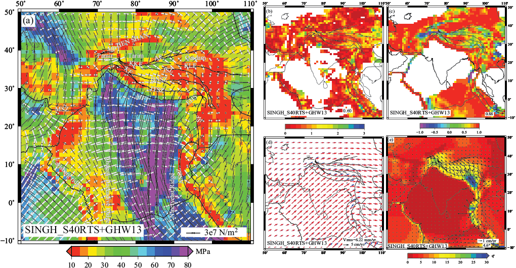
Fig. 1 Parameters predicted from combined model of GPE and mantle tractions derived from SINGH_S40RTS+GHW13 and their comparisons with observables. (a) Deviatoric stresses plotted on top of second invariant of deviatoric stresses. The compressional stresses are denoted by solid black arrows, while white arrows show tensional stresses, (b) Total misfit between predicted and observed SHmax from WSM. (c) Correlation between predicted stress tensors and GSRM strain rate tensors, (d) predicted (red) and observed plate velocities (blue), and (e) angular misfit between observed and predicted plate velocities; the arrows show vector difference between them. The average angular deviation (θ) is given in the bottom right of the figure. Published in Singh and Ghosh, 2020.
We also perform a quantitative comparison of our solutions to a range of surface observations such as plate velocities (Kreemer et al., 2014), strain rates from the Global Strain Rate Model (GSRM; Kreemer et al., 2014), and SHmax (most compressive principal stress axes) directions and style from World Stress Map (WSM; Heidbach et al., 2016) (Fig. 1b-e). We found that the coupled model of GPE and tractions derived from SINGH_S40RTS tomography model yielded the best fit to observations. The tomography model, SINGH_S40RTS resulted from embedding the local tomography model of Singh et al. (2014) in the global model of S40RTS (Ritsema et al. 2011). However, we observe significant misfits in velocities, especially in the IN-EU collision zone for this model, particularly near the eastern Himalayan syntaxis (EHS, see Fig. 1). Also, the correlation of deviatoric stresses with observed strain rates is observed to degrade near the Pamir and the eastern part of the Tibetan plateau (Fig. 1). Hence, we focused on the IN-EU collision zone to investigate possible reasons behind the misfits between the predicted and observed parameters.
Can the uncertainties in crustal structure be possible source of misfits?
To verify whether uncertainty in thickness and density of crustal layers contribute to the observed misfits as mentioned earlier, three crustal and lithospheric models, CRUST1.0, CRUST2.0 (Laske et al. 2001) and LITHO1.0 (Pasyanos et al. 2014) are tested for calculating GPE and associated deviatoric stresses using the FE model. LITHO performs better than both CRUST2 and CRUST1 in fitting the observations of SHmax, GSRM strain rates and plate velocities (Fig. 3). CRUST1 also matches the velocity in the IN-EU region better than CRUST2 and LITHO (Fig. 3, bottom panel). Hence, if we consider the CRUST1 and LITHO models, they alone are largely able of matching the observational constraints in this region. On the other hand, the predictions from CRUST2 are found to have large misfits, thus demonstrating the inability of CRUST2 model alone to constrain the deformation in this region.
How much of a role does mantle might play in these models?
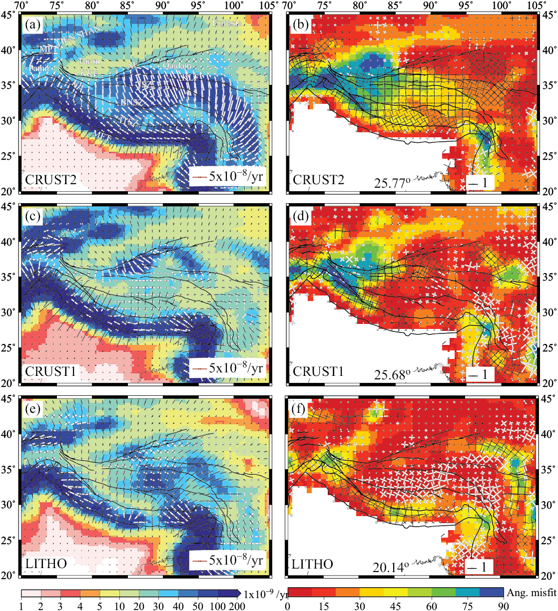
Fig. 2 Strain rates predicted from GPE only models plotted on top of their second invariants (left). The black arrows denote compression and white arrows represent extension. (Right) Difference between GSRM strain rates and those predicted by GPE models plotted on top of the angular misfit between predicted and observed most compressional strain axes. The arrows on top represent the type of deformation required to match the observed strain rates. The magnitudes of these arrows are scaled by the difference in regime (R) between observed and predicted strain rates. Published in Singh and Ghosh 2020.
In order to further constrain the relative contribution of the mantle, we computed the strain rates based on the predicted deviatoric stresses. All crustal models predict high strain rates along the Himalayas (>200 × 10-9), with large NE-SW compression (Fig. 2, left-hand column). Such high strain rates are also observed along both the eastern and western syntaxes. In order to quantify the type of deformation needed for matching the GSRM strain rates, we subtract the strain rates predicted by the crustal models from the GSRM strain rates. These residual strain rates indicate as to how much and what kind of strain is required from the mantle contribution to fit the GSRM strain rates. We find that strain rates predicted by CRUST2 require a large amount of compression to match the GSRM strain rates (Fig. 2b), as evident by the drastic improvement in fit to observations on adding large compressional stresses from S40RTS and SAW642AN models (Fig. 3). The strain rates predicted by CRUST1 suggest that it requires a large compressional strain in western Tibet to match the observed deformation (Fig. 2d). Mantle convection models predict large compression within this area due to subducted slabs in the underlying mantle. Hence adding the contribution from mantle convection models improves the fit significantly (Fig. 3). On the other hand, in central Tibet CRUST1 requires very small strain to match the GSRM strain rates (Fig. 3d). As LITHO predicts large N-S compression within central Tibet (Fig. 2e), extension is required that can reduce/cancel out the compression in order to match the observed deformation (Fig. 2f). However, the mantle convection models do not predict extension in this area, hence no significant changes are observed for LITHO model in central Tibet on adding the contribution from mantle. Both CRUST1 and LITHO require extension around the EHS to match the observed strain rates, as both models predict this area to be in thrust regime. Thus, the GPE only models require significant contribution from mantle in order to match the observed deformation.
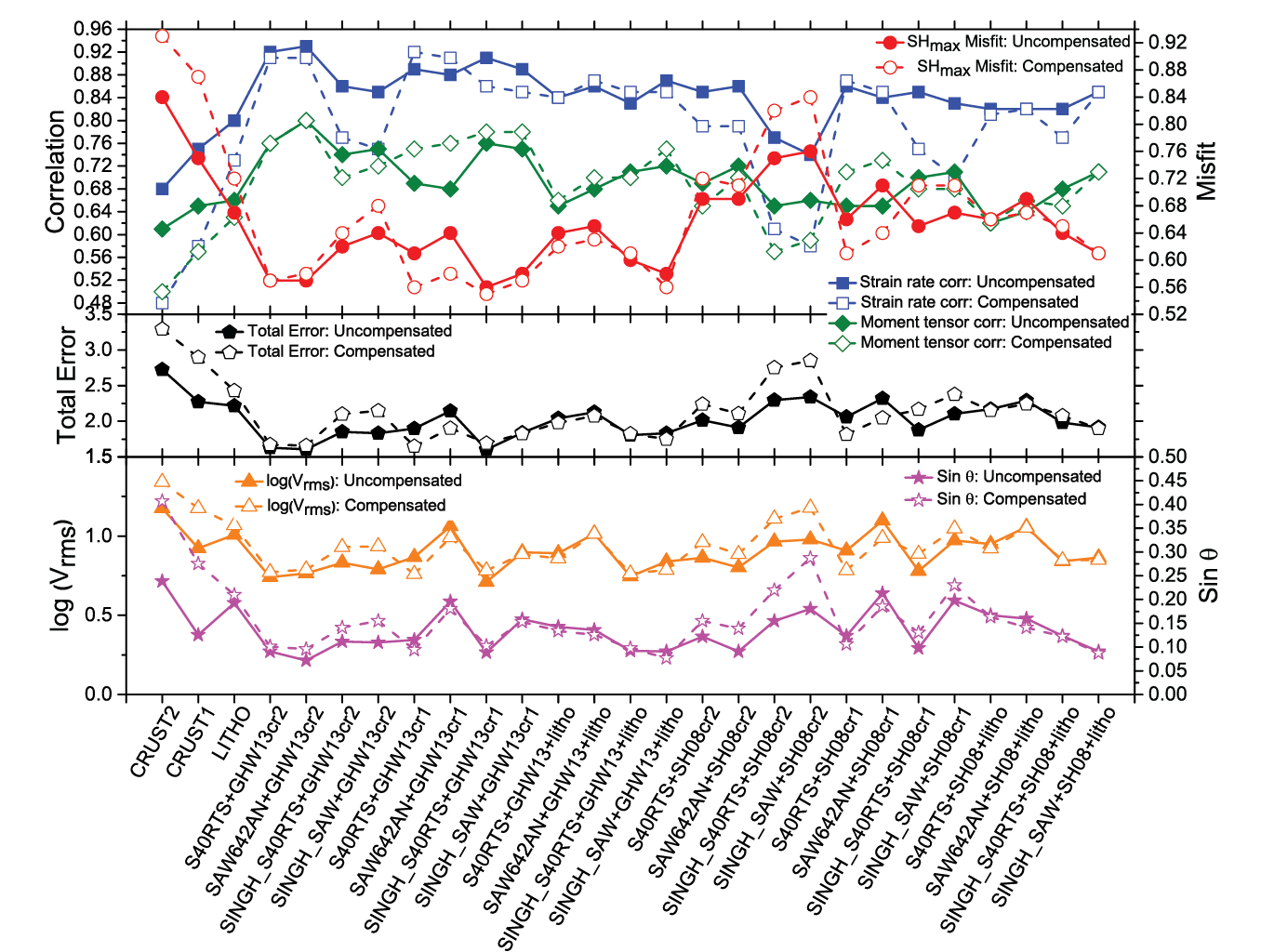
Fig. 3 Top panel shows plot of the correlation and misfits between observations and predictions for various models. The solid symbols represent uncompensated models, while open symbols are used for compensated models. Red represents the misfit between observed and predicted SHmax, while blue and green show the correlation of predicted deviatoric stress tensors with GSRM strain rates and moment tensors, respectively. The middle panel shows plot of total error for different models. The bottom panel shows log of rms error (orange) and sine of angular misfits (θ) (magenta) between observed and predicted velocities. Published in Singh and Ghosh, 2020.
Adding the mantle contribution
To compute mantle traction, we used density anomalies from S40RTS and SAW642AN tomography models along with their hybrid counterparts, SINGH_S40RTS and SINGH_SAW, which are obtained by embedding the Singh et al. (2014) tomography model in these global models, respectively. The mantle tractions are computed from these models for two radially varying viscosity structures using HC convection code. The stresses associated with these tractions are then added to those obtained from GPE only models, to account for both the sources of deformation in this region. Adding the contribution from mantle tractions improved the fit to surface observations for all three crustal models, but most prominently for CRUST2.
Thus, in our recent study (Singh and Ghosh, 2020), we suggest that a coupled model of lithosphere and mantle density variations can successfully explain the observations of strain rates, stresses and plate motions within the Indian plate and India-Eurasia collision zone. We also found that the relative contribution of lithosphere versus mantle forces varies depending on the crustal model used. Therefore, the inaccuracies in determining lithosphere structure (density and thickness) will lead to inaccuracies in estimating the relative contribution of these forces. Hence, an accurate crustal model is essential when trying to understand deformation.
References
England & Houseman. 1989. J. Geophys. Res. 94(B12), 17561-17579.
Flesch et al. 2001. J. Geophys. Res. 106(B8), 16435-16460.
Forte et al. 2010. Earth Planet. Sci. Lett. 295(3), 329-341.
Ghosh et al. 2006. Geology, 34(5). 321-324.
Ghosh et al. 2008. Geo. Res. Lett. 35, L16309.
Ghosh & Holt. 2012. Sci. 335(6070), 838–843.
Ghosh et al. 2013. J. Geophys. Res.- Sol. Ea. 118, 346-368.
Ghosh et al. 2013b. Geophys. J. Int. 194(2), 651-669.
Hager & O’Connell. 1981. J. Geophys. Res. 86(B6), 4843-4867.
Heidbach et al. 2016. WSM Team (2016): World Stress Map Database Release 2016. GFZ Data Services.
Kreemer et al. 2014. Geochem., Geophys., Geosys. 15, 3849-3889.
Laske et al. 2001. http://mahi.ucsd.edu/Gabi/rem.dir/crust/crust2.html.
Laske et al. 2013. Geophy. Res. Abs. 15, 2658.
Pasyanos et al. 2014. J. geophys. Res., 119(3), 2153-2173.
Ritsema et al. 2011. Geophys. J. Int. 184(3), 1223-1236.
Singh et al. 2014. Geochem., Geophys., Geosys. 15, 658-675.
Singh and Ghosh. 2020. Geophys. J. Int. 223, 111 - 131.
Steinberger & Holme. 2008. J. Geophys. Res. 113, B05403


Navneet Kumar
Very nice read