
Dr. Elodie Kendall, Postdoc in the Geodynamic modelling section of GFZ Potsdam
In this week’s News & Views, Postdoc Elodie Kendall from GFZ Potsdam shares with us recent work on the mantle structures that could explain the Indian Ocean Geoid Low.
What is the geoid, what does it look like and what can it tell us about mantle structure?
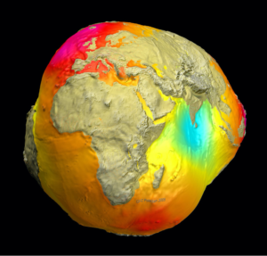
Figure 1: The geoid, also known as “Potsdam Gravity Potato” (data based on satellite LAGEOS, GRACE and GOCE and surface data, airborne gravimetry and satellite altimetry, as well as on the long-term data series, (image: GFZ, 2011).
The geoid is a model of the shape of the oceans’ surface if only gravity and Earth’s rotation acted on it and continued through the continents (the gravitational equipotential surface of Earth). Due to the uneven distribution of mass throughout the Earth, the geoid’s shape is smooth but irregular, as depicted by the famous Potsdam gravity potato in Fig. 1. These mass excesses and deficits lead to geoid anomalies with respect to the reference hydrostatic ellipsoid of +85 m to -106 m (GRACE).
Long wavelength geoid anomalies have their origin in the Earth’s mantle and provide important constraints on the density and viscosity structure of the Earth’s interior. One of the most pronounced geoid lows on Earth lies just south of the Indian peninsula. When shown relative to hydrostatic equilibrium, and corrected for the crust and mid-ocean ridges, it appears as merely a regional low on a north-south trending belt of low geoid (Fig. 2a).
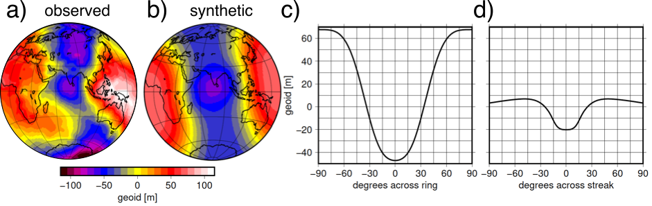
Figure 2: a) Observed geoid (Pavlis et al., 2012) relative to equilibrium spheroid (Nakiboglu, 1982) minus contribution of crust from CRUST1.0 (Laske et al., 2013), minus the effect of ocean floor age (Müller et al., 2008) following Steinberger (2016) and assuming isostatic compensation. b) Synthetic geoid built from a high (0.5%) density anomaly (ring-shape; ~N-S trending; half-width 15 degrees, between 1500 and 2600 km depth) in the lower mantle and a low density (-0.7%) anomaly (a streak; ~E-W trending; half-width 7 degrees, between 100 and 400 km depth) in the upper mantle. c and d) Orthogonal profiles through the ring and streak density anomalies, respectively. The effect of the olivine-spinel phase transition is considered.
How well can we model the observed geoid?
The effect of density anomalies at a given depth and spherical harmonic degree on the geoid can be expressed in terms of geoid kernels (i.e., how sensitive the geoid is to density variations with depth; Richards and Hager, 1984; Ricard et al., 1984). Figure 3 shows that for long wavelengths (i.e., focusing solely on degree 2 & 3 in red and orange), these kernels reverse sign in the lower mantle. Below ~1500 km, the kernel is negative such that a positive density anomaly in the lower part of the mantle would give rise to a negative geoid. In the upper mantle the kernel is positive and a negative density anomaly would give rise to a negative geoid.
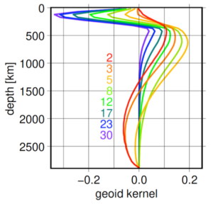
Figure 3: Geoid kernels for spherical harmonic degrees 2, 3, 5, 8, 12, 17, 23, 30 for the reference viscosity structure from Steinberger (2016). The kernels show the sensitivity of the geoid to density anomalies with depth.
Recently, Ghosh et al. (2017) showed that the Indian Ocean Geoid Low (IOGL) can be explained well by density anomalies inferred from seismic tomography, but the cause of these density anomalies was not thoroughly investigated. Therefore, we pursue the idea stemming from Ghosh et al. (2017) that the IOGL occurs at the crossing point of a roughly north-south trending positive anomaly “ring” in the lower mantle (e.g. slabs from the “ring of fire”) and a roughly east-west to WSW-ENE trending negative anomaly “streak” in the upper mantle (see Fig. 2), by developing a set of simple, synthetic geoid/density models (Steinberger et al., 2021).
We show that with realistic assumptions we can approximately match the size, shape and magnitude of the geoid low (Fig. 2b, from a combination of a high-density “ring” in the lower mantle and a low-density “streak” in the upper mantle from East Africa in a east-north-east direction. The modelled geoid built with these parameters (Fig. 2c,d) reproduces the overall size and shape of the actual geoid low of -30 m (relative to the “saddle” to the north) or -50 m (relative to the “saddle” to the SE), on an extended roughly north-south trending geoid low. Please see Steinberger et al. (2021) for more information about the methodology and sensitivity of the geoid to the size and depth extent of the density structures.
Where could hot anomalies in the upper mantle beneath the West Indian ocean come from?
To address this question, we consider that the IOGL is slightly elongated towards East Africa (Fig. 2a), which could correlate with an outflow from the Kenya plume rising from the margin of the African LLSVP, as imaged by current tomography models (Chang et al., 2020, 2015; Durand et al., 2017; Boyce et al., 2021). Evidence for a hot mid-mantle anomaly in the area of the IOGL has also been reported by Reiss et al. (2017) and Rao et al. (2020) who used seismic data to reveal a thin mantle transition zone. Moreover, in light of previous et al. (2005) suggested that it is implausible for the African LLSVP to tilt all the way to Afar. As the IOGL is even further from South Africa than Afar, we find it even more plausible here that material is channelled in the upper mantle from the Kenya plume.
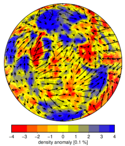
Figure 4: Average density in the depth range 100-400 km and flow field at depth 262.5 km for the reference model of Steinberger (2016). 10 degrees of arc arrow length = 5 cm/yr.
In Fig. 4 we show the present-day mantle flow field at 262.5 km depth and the average density anomaly in the upper mantle from a recent tomography-based model (Steinberger, 2016). It shows a series of low-density material which, in combination with the arrows showing horizontal flow, could indicate an outflow from the Kenya plume towards the southern tip of India. A transition from eastward towards more north-eastward flow further east could be due to the strong northward component of the Indian plate motion dragging material along. The low-density anomaly correlates well with a linear low S-velocity anomaly east of East Africa in the votemap (Hosseini et al., 2018; Shephard et al., 2017) of many tomographic models and in the isosurfaces of current global tomography models such as SGLOBE-rani (Chang et al., 2015), SAVANI (Auer et al., 2014), SEISGLOB2 (Durand et al., 2017) and S362ANI (Kustowski et al., 2008) (Fig. 5). Figure 4 and maps of lithospheric thickness beneath Africa (Globig et al., 2016) show a region of thicker lithosphere beneath the Horn of Africa (Somalia). Therefore, flow may be diverted around regions of thick lithosphere and focused in regions of thinner lithosphere such as north of Madagascar. All in all, we propose that the IOGL could be caused by a high-density anomaly in the lower mantle and hot material in the upper mantle supplied by the Kenya plume in the west, a plume-slab overpass.
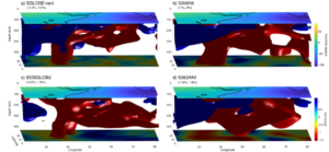
Figure 5: Isosurfaces of low- and high-velocity anomalies in the upper mantle beneath East Africa and the Indian Ocean from four global tomography models; SGLOBE-rani (Chang et al., 2015), SAVANI (Auer et al., 2014), SEISGLOB2 (Durand et al., 2017) and S36ANI (Kustowski et al., 2008). We used different values for isosurfaces in each model to clearly show the lowest-velocity anomalies, which are noted on the top left of each subplot.
References

Auer et al. 2014. J. Geophys. Res. - Sol. Ea. 119, 3006–3034.
Boyce et al. 2021. Geochem., Geophys., Geosys. n/a, e2020GC009302.
Burke et al. 2008. Earth Planet. Sci. Lett. 265, 49–60.
Chang & Van der Lee 2011. Earth Planet. Sci. Lett., 302 (3-4), 448–454.
Chang et al. 2015. J. Geophys. Res. - Sol. Ea. 120, 4278–4300.
Chang, Kendall, Davaille, Ferreira 2020. J. Geophys. Res. - Sol. Ea. 125, e2020JB019929.
Davaille et al. 2005. Earth Planet. Sci. Lett. 239, 233–252.
Durand et al. 2017. Geophys. J. Int. 211, 1628–1639.
"Earth's Gravity Definition". GRACE - Gravity Recovery and Climate Experiment. Center for Space Research (University of Texas at Austin) / Texas Space Grant Consortium. 11 Feb 2004. Retrieved 22 Feb 2021.
Ghosh et al. 2017. Geophys. Res. Lett. 44, 9707–9715.
Globig et al. 2016. J. Geophys. Res.- Sol. Ea. 121, 5389–5424.
Hager & O’Connell 1979. J. Geophys. Res. 84, 1031–1048.
Hager & O’Connell 1981. J. Geophys. Res. 86, 4843–4867.
Hosseini et al. 2018. Geochem., Geophys., Geosys. 19, 1464–1483.
Kustowski et al. 2008. J. Geophys. Res. 113, B06306.
Laske et al. 2013. Geophys. Res. Abstr. 15. Abstract EGU2013-2658.
Müller et al. 2008. Geochem., Geophys., Geosys. 9, Q04006.
Nakiboglu 1982. Phys. Earth Planet. Inter. 28, 302–311.
Rao & Kumar 2014. Phys. Earth Planet. Inter. 236, 52–59.
Rao et al. 2020. Geochem., Geophys., Geosys. 21, e2020GC009079.
Reiss et al. 2017. Geophys. Res. Lett. 44, 6702–6711.
Ricard et al. 1984. Ann. Geophys. 2, 267–286.
Richards & Hager 1984. J. Geophys. Res. 89, 5987–6002.
Pavlis et al. 2012. J. Geophys. Res. 117, B04406.
Shephard et al. 2017. Scientific Reports 7, 10976.
Steinberger & Calderwood 2006. Geophys. J. Int. 167, 1461–1481.
Steinberger, B., Rathnayake, S., Kendall., E. 2021. The Indian Ocean Geoid Low at a plume-slab overpass. Earth and Space Science Open Archive preprint, submitted to Tectonophysics.
Yuan & Beghein 2013. Earth  Planet. Sci. Lett. 374, 132–144.


Charles Aker
Earth’s akin to plum pudding, with nickel for plums 🤫
OUZZAOUIT MOULAY ABDELLOIHD
très intéressant