Mantle flow and deformation beneath tectonic plates
From geodynamics 101 you probably know that the thermal evolution of oceanic lithosphere is well-described by the plate cooling model where a rigid oceanic plate thickens as a function of its age as it moves away from the ridge axis. However, surprisingly, no such depth-age trend is observed for radial anisotropy! A mystery that I will not leave you pondering on, but instead I will discuss it later in this blog post.
How and what do we know about mantle flow and deformation beneath tectonic plates ?
Dr. Elodie Kendall is a Postdoc in the ERC project “Meet” in the Geodynamic modelling section of GFZ Potsdam. Here she shares with us her recently published work on the role of plate speed on the development of the radial anisotropy.
The asthenosphere experiences large deformation and is a key control on present day plate motions. During deformation such as from plate motion, grains of olivine, the main rock forming mineral in the asthenosphere, rotate into a preferred direction parallel to the deformation, developing a texture that can be measured seismically. For example, seismic radial anisotropy is the squared ratio between the speeds of horizontally- and vertically polarized shear waves, ξ= VSH2/VSV2. ξ>1 (VSH2>VSV2) indicates to first order horizontal flow in the upper mantle.
The asthenosphere is thought to primarily deform in the so-called dislocation and diffusion creep regimes (e.g., Karato, 1993). The former regime is expected to result in observable seismic anisotropy. Relative motion of the overlying plate controls tectonic stress and the creep regime and therefore the strength of seismic anisotropy. While previous studies have predicted radial anisotropy that fits with observations (e.g., Auer et al., 2015; Hedjazian et., al 2017), in this blog I illustrate the results of our new study (Kendall et al., 2022) on the role of the plate speed on the development of radial anisotropy beneath the oceans.
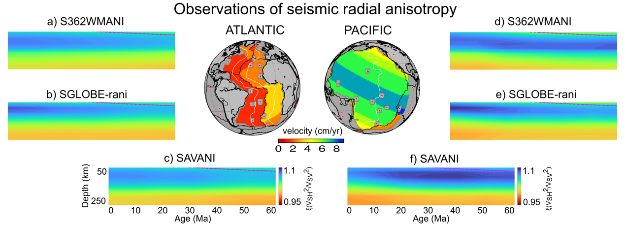
Figure 1 : Various seismic anisotropy models (S362WMANI, Kustowski et al., 2008; SGLOBE-rani, Chang et al., 2015; SAVANI, Auer et al., 2014) beneath the slow Atlantic plate (left) and the faster Pacific plate (right).
In Figure 1 I present three global anisotropic mantle models which have been built using millions of seismic waves and are sensitive to the asthenosphere. Blue colours (radial anisotropy, ξ>1) indicate (to first order) horizontal flow in the oceanic asthenosphere. In our new study, we propose that the intensity of the radial anisotropy increases with plate speed (Kendall et al., 2022). For example, higher radial anisotropy is observed beneath the Pacific (Figure 1d-f), moving at an average speed of 8 cm/yr compared to the the Atlantic plate (Figure 1a-c) which is moving at on average at 2 cm/yr. In our study, we also ran additional tests to ensure that the seismic resolution beneath both plates are similar and therefore can be compared.
Why is seismic anisotropy different beneath different oceans?
In order to address this question, we simulated surface-driven mantle flow beneath an oceanic plate solving sets of physical equations using the finite difference code I2VIS (Gerya and Yuen, 2003). Figure 2 (a and f) shows the initial setup with a ridge-axis on the left-hand side, a subduction zone on the right and we apply a constant velocity of 2 or 8 cm/yr to represent slow (e.g., Atlantic) and fast plates (e.g., Pacific), respectively. For more details, all physical and rheological parameters are described in Kendall et al., 2022.
Then, we model the development of seismic anisotropy using a modified version of the kinematic model, D-Rex (Kaminski et al. 2004). The second, third and fourth row of Figure 2 shows stress, dominant deformation mechanism and predicted radial anisotropy beneath the slow and fast plate. Faster plate motion leads to higher tectonic stresses, resulting in more deformation in the dislocation creep regime (which leads to seismic anisotropy) and deeper radial anisotropy than beneath the slow plate.
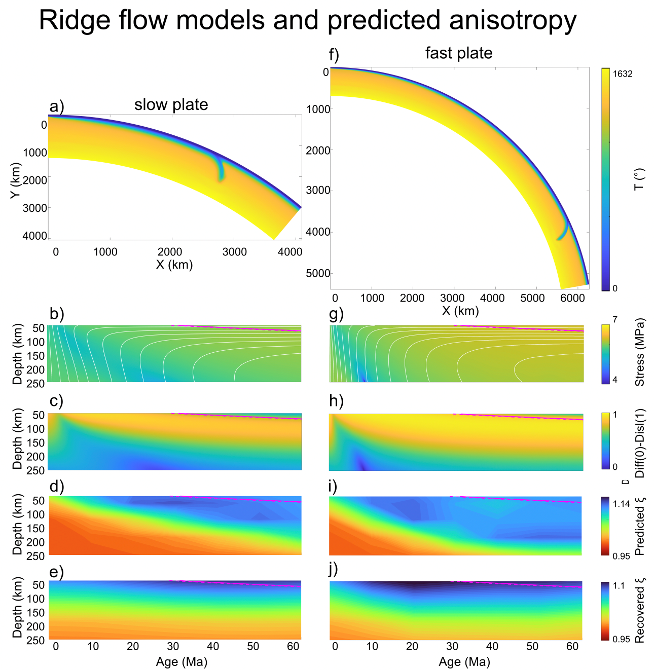
Figure 2 : Top row to bottom row: Temperature, stress, fraction of diffusion to dislocation creep, predicted and recovered seismic anisotropy after application of the tomographic filter for the slow (left) and fast (right) plate model.
Can we more fairly compare observations and predictions of seismic structure?
For a fair comparison between predictions and observations of seismic anisotropy we project the synthetic structure as seismic images using a tomographic filter. I.e., we take into account the incomplete data coverage, model parameterization (e.g., the functions used to describe horizontal and vertical seismic variations) and regularization (imposing additional constraints on the problem to help stabilise inversions).
Figure 2e and j, fourth row and the top row of Figure 3 (a and e) shows that deeper anisotropy beneath the faster oceanic plate has translated into stronger anisotropy and that the depth-age dependence of anisotropy is not recovered when applying the tomographic filter, in line with observations. While some people propose that the flat depth-age relation is due to some physical mechanism, we wanted to check that it wasn’t just due to strong regularization that are used in some tomography models. Sure enough it looks to play a strong role.. Stronger regularization (e.g., Figure 3, from bottom to top) limits seismic anomalies closer towards the reference model, PREM (a 1D profile with no radial anisotropy beneath 220km depth), therefore flattening the depth-age trend. Models with weak regularization are able to recover a depth-age trend in radial anisotropy!
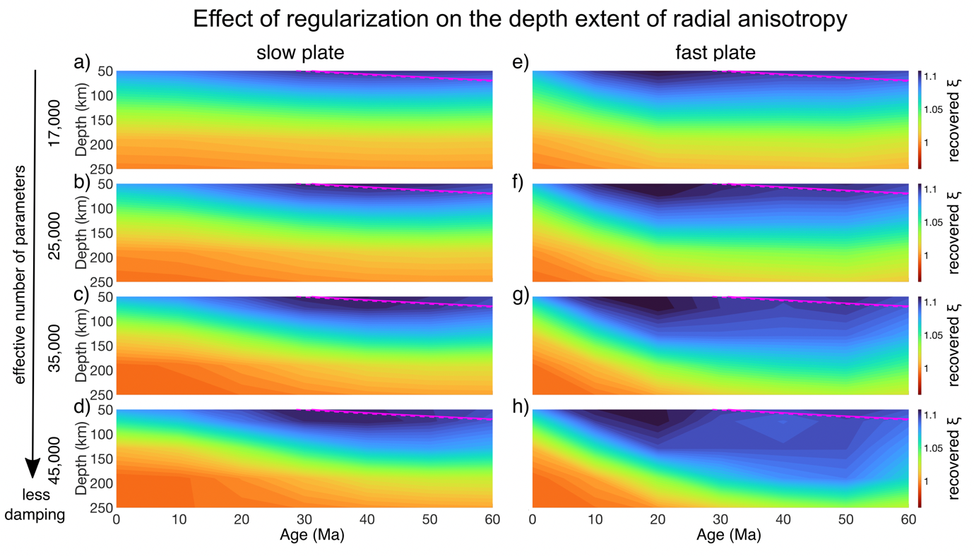
Figure 3 : Seismic anisotropy as a function of ocean-floor age for the slow (left) and fast (right) oceanic plate. Strong regularization/damping can flatten a depth-age trend (bottom to top).
To conclude, as oceanic plate speed increases from 2 cm/yr to 8 cm/yr, observed and predicted radial anisotropy increases by ~0.01-0.025 in the upper 100-200km of the mantle between 10-60Ma. This study was important to understand the relation between oceanic plates and induced deformation (as summarised in Figure 4) but it can also aid research of other more complex mechanisms of generating seismic anisotropy, such as from melts.
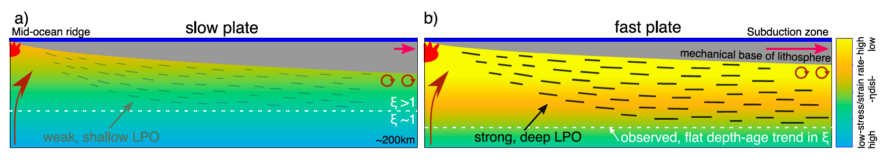
Figure 4 : Schematic of the proposed mechanism such that higher tectonic stresses/strains (background colour) beneath faster plates lead to lower dislocation creep viscosities and therefore deeper radial anisotropy, (shown by black bars) than beneath slower plates. After tomographic inversion, this deeper anisotropy translates into simply stronger anisotropy and the depth-age trend is lost with strong regularization.
Auer, L., Boschi, L., Becker, T., Nissen-Meyer, T., and Giardini, D. (2014). Savani: A variable resolution whole-mantle model of anisotropic shear velocity variations based on multiple data sets. Journal of Geophysical Research: Solid Earth, 119:3006-3034.

Auer, L., Becker, T. W., Boschi, L., and Schmerr, N. (2015). Thermal structure, radial anisotropy, and dynamics of oceanic boundary layers. Geophysical Research Letters, 42:9740-9749.

Beghein, C., Yuan, K., Schmerr, N., and Xing, Z. (2014). Changes in Seismic Anisotropy Shed Light on the Nature of the Gutenberg Discontinuity. Science, 343:1237-1240.

Burgos, G., Montagner, J.-P., Beucler, E., Capdeville, Y., Mocquet, A., and Drilleau, M. (2014). Oceanic lithosphere-asthenosphere boundary from surface wave dispersion data. Journal of Geophysical Research: Solid Earth, 119:1079-1093.

Chang, S.-J., Ferreira, A. M. G., Ritsema, J., van Heijst, H. J., and Woodhouse, J. H. (2015). Joint inversion for global isotropic and radially anisotropic mantle structure including crustal thickness perturbations. Journal of Geophysical Research: Solid Earth, 120(6):4278-4300.

Gerya, T. V. and Yuen, D. A. (2003). Characteristics-based marker-in-cell method with conservative finite-differences schemes for modeling geological flows with strongly variable transport properties. Physics of the Earth and Planetary Interiors, 140:293-318.

Hedjazian, N., Garel, F., Davies, D. R., and Kaminski, E. (2017). Age-independent seismic anisotropy under oceanic plates explained by strain history in the asthenosphere. Earth and Planetary Science Letters, 460:135-142.

Kaminski, E., Ribe, N. M., and Browaeys, J. T. (2004). D-Rex, a program for calculation of seismic anisotropy due to crystal lattice preferred orientation in the convective upper mantle. Geophysical Journal International, 158:74-752.

Karato, S.-I. (1993). Importance of anelasticity in the interpretation of seismic tomography. Geophysical Research Letters, 20(15):1623-1626.

Kendall, E., Faccenda, M., Ferreira, A.M., & Chang, S.-J. (2022). On the relationship between oceanic plate speed, tectonic stress and seismic anisotropy. Geophysical Research Letters, 49, e2022GL097795. https://doi.org/10.1029/2022GL097795

Kustowski, B., Ekstrom, G., and Dziewonski, A. M. (2008). Anisotropic shear-wave velocity structure of the Earth's mantle: A global model. Journal of Geophysical Research: Solid Earth, 113:B06306.