Is the lower mantle boring?
For a long time, the lower mantle was thought to be relatively featureless and uniform compared to the more dynamic upper mantle. But recent seismic observations are challenging that idea, especially when we look near the base of the mantle. Recent studies from Maureen Long’s group (Creasy et al. 2017, Wolf et al. 2019, Reiss et al. 2019, Wolf & Long, 2023) and others (Cottar & Romanowicz 2013, Asplet et al., 2023) have shown that seismic waves at the base of the mantle don’t travel the same way in all directions. This effect, called anisotropy, hints that the lowermost mantle is far from uniform and might be more dynamic than we once thought. These seismic signatures are strikingly different from the rest of the mantle. And from a geodynamics point of view, that’s exciting because it suggests something unusual is happening with how materials flow or deform near the core-mantle boundary.
This is exactly what got me hooked: what if the base of the mantle holds the key to understanding deep mantle flow? Does it help to know more of the dynamics of the mantle plumes? In this blog post, I’ll take you through why the lowermost mantle is far from boring and why geodynamicists and seismologists alike are increasingly drawn to this mysterious region just above the core.
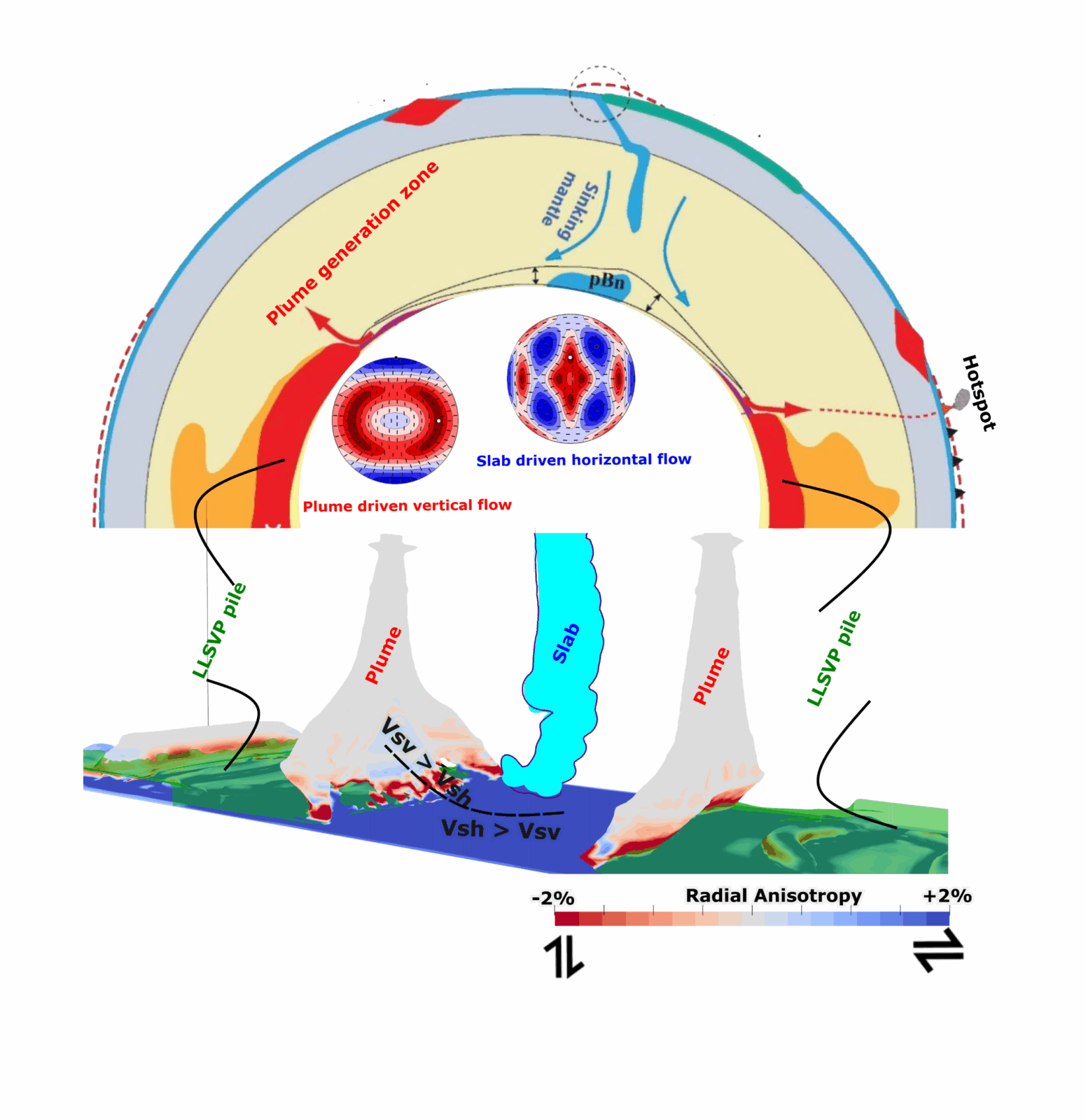
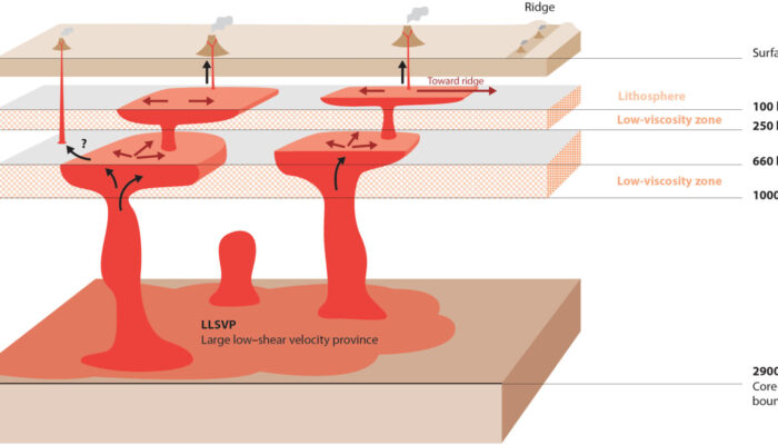
Figure 1: How the deep mantle “talks” to the surface. The top panel shows the big-picture circulation of the lower mantle (adapted from Torsvik et al. 2016), while the bottom zooms in on flow patterns near the core-mantle boundary (adapted from Roy et al. 2025). To decode these flows, we look at two key minerals bridgmanite and post-perovskite whose seismic “fingerprints” (pole figures) reveal which directions waves move fastest or slowest (middle panel). Together, these snapshots link mantle dynamics to the signals measure by seismologists.
What we know from seismology?
For more than two decades, seismologists have known that the lowermost mantle isn’t uniform. Early studies (e.g. Garnero & McNamara 2008; Burke et al., 2008) proposed the existence of two continent-sized “blobs” of dense material sitting just above the core; one beneath Africa and one beneath the Pacific. These regions are now widely known as LLSVPs (Large Low Shear Velocity Provinces), because seismic waves slow down dramatically as they pass through them (Lekic et al 2012).
With advances in seismology, we’ve been able to zoom in on these structures in greater detail. It’s not just about whether waves travel faster or slower; it’s also about whether they behave differently depending on their direction of travel. This property, called seismic anisotropy, is especially strong around the margins of LLSVPs and near the roots of plumes and slabs at the base of the mantle. In other words, anisotropy gives us new, finer-scale clues about how the lowermost mantle works.
But here’s the challenge: seismology alone gives us snapshots; wave speeds and temperature anomalies. Cold regions show up as fast, hot regions as slow. What we don’t get is the movie: the flow patterns of mantle material, the continuous motion and deformation that shapes those signals.
That’s where geodynamics steps in. By running numerical models of mantle flow, and linking them to how minerals align (which seismologists detect as anisotropy), we can move beyond static snapshots to actually reconstruct the hidden dynamics of Earth’s deepest interior. And that’s exactly what motivated me: to investigate, geodynamically, what could be causing the anisotropy observed at the base of the mantle.
What did we do to investigate this?
Since we can’t dig down to the core-mantle boundary (CMB), we turned to computer simulations to see what might be happening down there. Our goal was simple: understand what could generate the seismic anisotropy observed in seismic studies.
Simulating mantle flow
First, we created a series of geodynamic models using the open-source code ASPECT (Heister et al. 2017) that mimic how the mantle moves over time. These models allowed us to explore how downwelling slabs could reach the CMB, perturb the thermal boundary layer at the base of the mantle, and generate upwelling flow from the edges of the LLSVP piles.
Tracking mineral alignment
Next, we focused on the minerals that make up most of the lowermost mantle: bridgmanite and post-perovskite. Using a method called D-REX by utilizing the open-source code ECOMAN (Faccenda et al., 2024), we simulated how these minerals align under the forces of mantle flow which is called the crystal preferred orientation (CPO) (Figure 2). Why does this matter? Because the alignment of minerals controls how seismic waves split in different directions, essentially encoding the flow patterns into the anisotropic signals we detect at seismic observation.
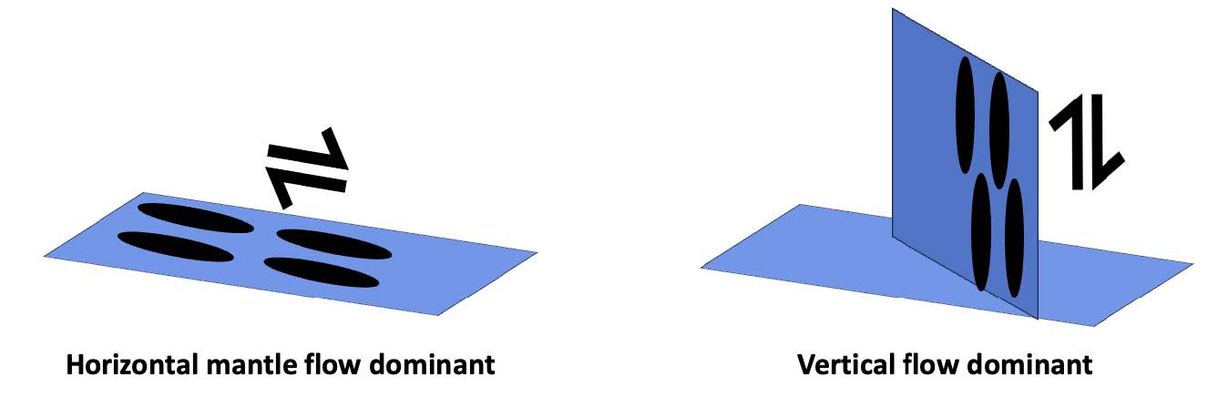
Figure 2: A simple sketch of how mantle flow is determined: mineral grains (black ellipses) deep in the mantle tend to line up in certain directions (their “crystal preferred orientation”), and this alignment lets us read the flow of the mantle like a fingerprint. This schematic shows a simplified case, based on the active slip systems of minerals considered in Roy et al. (2025), which best fits seismic observations. Flow patterns can look different if other slip systems are active; see the supplementary section of Roy et al. (2025) for details.
Testing different conditions
We have tested several properties like temporal evolution of plume surfacing events in the form of earlier versus later stages of plume formation, effect of thermal conductivity, stress exponent, strength of LLSVP, viscosities of ambient mantle, influence of the presence of a slab, morphological differences between thermochemical (presence of LLSVP) and thermal (no LLSVP) plumes and their effects on the anisotropic signature of mantle plumes (Figure 3).
This allowed us to explore a range of possibilities: What happens when cold slabs hit the base of the mantle? How do hot plumes rise from the edges of LLSVPs? How does mineral alignment and therefore seismic anisotropy change under different flow regimes? What would be the flow pattern if there is no slab influence on plume formation? What could be the flow regime without the presence of LLSVP piles?
Connecting models with observations
With D-REX modelling (see our related article) , we can track how mantle minerals align. From this, we calculate shear wave radial anisotropy ξ = V2SH/V2SV; a measure of whether seismic waves move faster horizontally or vertically, with positive ξ – 1 > 0 indicating faster horizontal shear waves and negative is vice-versa (Figure 3). With the slip systems we used for bridgmanite and post-perovskite, positive radial anisotropy means the rocks are shearing horizontally, while negative anisotropy points to vertical shearing – a clue to how the mantle is actually flowing down there. We then calculate the shear wave azimuthal anisotropy (Figure 4) which refers to the variation of wave velocity as a function of the azimuthal propagation direction (the horizontal angle) relative to a reference direction. In simple words, azimuthal anisotropy shows the directions in which seismic waves move fastest – a sort of compass that points to the direction of mantle flow.
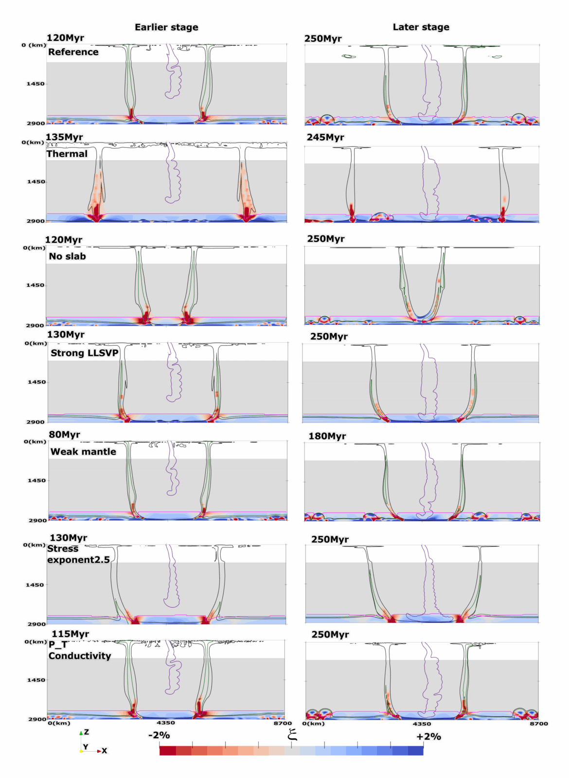
Figure 3: How anisotropy evolves with mantle plumes: This snapshot shows how shear wave anisotropy develops as plumes rise from the base of the mantle. On the left, you see an earlier stage of plume evolution; on the right, a later stage. The black outlines track the hot plumes, while purple marks the slab and green the LLSVP piles. The pink line shows the bridgmanite to post-perovskite phase transition boundary (Roy et al. 2025).
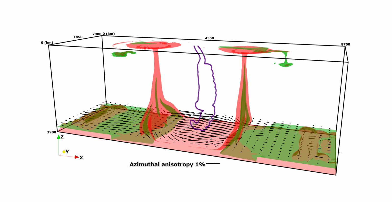
Figure 4: Azimuthal anisotropy around mantle plumes: The black lines show how the orientation of seismic waves (the fast polarization directions) shifts from the surrounding slab to the roots of the plumes at 2650 km depth. Red marks the rising plumes, purple the cold slabs, and green the LLSVPs. This snapshot comes from our reference model after 250 million years of mantle evolution, showing how mineral alignment in the deep Earth leaves a clear seismic fingerprint (Roy et al. 2025).
This integrated workflow (Roy 2024, Roy et al. 2025) allows us to produce predictions that can be directly compared with what seismologists observe, helping us build a clearer picture of Earth’s lowermost mantle, even in a region where direct observations remain scarce.
By comparing our simulations with seismic data, we could explain the way minerals align in these flows and why seismic waves travel faster or slower in certain directions, leading to the clue to the unseen dynamics of our planet’s deepest reaches.
Main-takeaways
Our results reveal some striking patterns: mantle plumes are robust generators of anisotropic signals, especially fast vertical shear wave velocities (Vsv) near the base of the mantle. On the slab side, we see widespread strong positive radial anisotropy (Vsh > Vsv), while on the LLSVP (pile) side, the signal varies from sometimes positive to sometimes nearly isotropic, depending on the rheological contrast (Figure 3). When considering azimuthal anisotropy, flow can be deflected near-perpendicularly from the base of the slab towards the generation of mantle plume zones (Figure 4). This shows that seismic anisotropy can act like a diagnostic tool, offering clues about the flow pattern which shapes the rheology and composition of deep Earth structures. These insights bring us one step closer to connecting what we see in seismic data with what’s really happening deep inside our planet, far below the surface. Our findings don’t just explain curious seismic signals, they also give us new ways to pinpoint where slabs sink and plumes rise, and to better constrain the strength and behavior of the dense LLSVP piles at the base of the mantle.

Poulami Roy
In this project, I was lucky to work with Bernhard Steinberger, Manuele Faccenda, and Michael Pons. From Bernhard, I picked up a lot about how the lower mantle actually works; with Michael, I built the geodynamic models that let us explore those dynamics; and from Manuele, I learned how seismic anisotropy can reveal the flow patterns of Earth’s mantle.
References

Creasy, N., Long, M. D., & Ford, H. A. (2017). Deformation in the lowermost mantle beneath Australia from observations and models of seismic anisotropy. Journal of Geophysical Research: Solid Earth, 122 (7), 5243–5267.

Wolf, J., Creasy, N., Pisconti, A., Long, M. D., & Thomas, C. (2019). An investigation of seismic anisotropy in the lowermost mantle beneath Iceland. Geophysical Journal International, 219 (Supplement 1), S152–S166.

Reiss, M. C., Long, M. D., & Creasy, N. (2019). Lowermost mantle anisotropy beneath Africa from differential SKS-SKKS shear-wave splitting. Journal of Geophysical Research: Solid Earth, 124 (8), 8540–8564.

Wolf, J., & Long, M. D. (2023). Lowermost mantle structure beneath the central Pacific Ocean: Ultralow velocity zones and seismic anisotropy. Geochemistry, Geophysics,Geosystems, 24 (6), e2022GC010853.

Cottaar, S., & Romanowicz, B. (2013). Observations of changing anisotropy across the southern margin of the African LLSVP. Geophysical Journal International, 195 (2),1184–1195.

Asplet, J., Wookey, J., & Kendall, M. (2023). Inversion of shear wave waveforms reveal deformation in the lowermost mantle. Geophysical Journal International, 232 (1), 97–114.

Torsvik, T. H., Steinberger, B., Ashwal, L. D., Doubrovine, P. V., & Trønnes, R. G. (2016). Earth evolution and dynamics—a tribute to Kevin Burke. Canadian Journal of Earth Sciences, 53(11), 1073-1087.

Roy, P., Steinberger, B., Faccenda, M., & Pons, M. (2025). Modeling anisotropic signature of slab-induced mantle plumes from thermochemical piles in the lowermost mantle. Geophysical Research Letters, 52 (10), e2024GL113299.

Garnero, E. J., & McNamara, A. K. (2008). Structure and dynamics of Earth's lower mantle. science, 320(5876), 626-628.

Burke, K., Steinberger, B., Torsvik, T. H., & Smethurst, M. A. (2008). Plume generation zones at the margins of large low shear velocity provinces on the core–mantle boundary. Earth and Planetary Science Letters, 265(1-2), 49-60.

Lekic, V., Cottaar, S., Dziewonski, A., & Romanowicz, B. (2012). Cluster analysis of global lower mantle tomography: A new class of structure and implications for chemical heterogeneity. Earth and Planetary Science Letters, 357, 68-77.

Heister, T., Dannberg, J., GassmÅNoller, R., & Bangerth, W. (2017). High accuracy mantle convection simulation through modern numerical methods - II: Realistic models and problems. Geophysical Journal International, 210 (2), 833–851.

Faccenda, M., VanderBeek, B. P., de Montserrat, A., Yang, J., Rappisi, F., & Ribe, N. (2024). Ecoman: an open-source package for geodynamic and seismological modelling of mechanical anisotropy. Solid Earth, 15 (10), 1241–1264.

Roy, P. (2024). Lower mantle anisotropy due to plume generation from Large Low-Shear-Velocity Provinces (Doctoral dissertation, Universität Potsdam).