Generation and reversal of the Earth’s magnetic field have remained one of the most controversial topics. In this week’s geodynamics 101, Debarshi Majumder, a PhD student from the Indian Institute of Science, gives a brief overview of the theory of geodynamo reversal and discusses some of the preliminary results obtained from numerical modelling.

A planetary magnetic reversal is one of the least understood topics in geophysics. The Earth’s magnetic field undergoes reversal repeatedly, but not periodically. The magnetic field of the Earth is generated by dynamo action in the liquid iron outer core (Labrosse, 2003). Dynamo action explains how a rotating, convecting, and electrically conducting fluid sustains a magnetic field. The outer core temperature is so high that iron can remain in a liquid state, which provides the essential ingredient for a dynamo. The driving force for the dynamo is a combination of thermal and compositional convection (Davies and Gubbins, 2011). The heat required for the thermal convection comes from secular cooling, latent heat release during solidification of iron at the inner core boundary, and possibly from radiogenic heat sources. The inner core is believed to have formed less than 1 billion years ago (Smirnov et al., 2011). Before the inner core formation, the convection is believed to have been thermal in nature. As the inner core solidifies, it releases lighter elements into the outer core fluid, generating compositional buoyancy. This compositional buoyancy is a key in driving the flow in outer core, which plays an essential role in sustaining and strengthening the geodynamo.
Mathematics of sustaining geomagnetism:
Let us look into the magnetic induction equation to understand how this magnetic field can remain strong over the years.
∂B/∂t=∇×(U×B) +η∇2B
There are two parts on the right-hand side of the equation. The first term [∇×(U×B)] is a magnetic field generation term. It describes the interaction between the magnetic field (B) and the flow velocity (U). The second term [η∇2B, η is the magnetic diffusivity] is the diffusion term, which causes decay to the magnetic field. Therefore, a steady-state magnetic field ∂B/∂t can be obtained if the sum of these two terms, i.e., the generation of the magnetic field and the decay of the magnetic field, becomes zero. This primary balance is needed for sustaining the planetary magnetic field.
Reasons of magnetic reversal
Apart from governing the flow of outer core fluid, the buoyancy also triggers the magnetohydrodynamic waves in the outer core in the presence of a rotating magnetic field. The primary force balance is present between Coriolis and pressure forces (geostrophic balance) in the outer core. However, the local force balance is present among magnetic, Coriolis, and Archimedean (buoyancy) forces (MAC balance) (Aubert, 2018). The buoyancy force modifies the magnetohydrodynamic waves significantly. If this buoyancy becomes large, it facilitates geodynamic reversal (Sreenivasan et al., 2014).
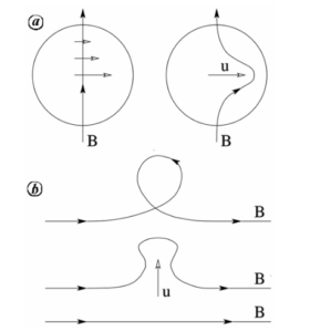
Figure 1: Schematic of the α-ωdynamo cycle (from Malkus 1978). (a) shows how a poloidal magnetic field (B) is transforming into a toroidal field due to a differential rotation (omega effect). (b) shows a toroidal magnetic field is generating poloidal field (alpha-effect)
One of the major characteristics of the geomagnetic field is that, the magnetic field is approximately dipolar in nature. Bullard and Gellman (1954) mentioned a cyclic process in which the poloidal magnetic field is generated by a toroidal magnetic field and vice versa. Differential rotation deforms the existing poloidal field and generates a toroidal magnetic field. This effect is known as the ω-effect. Whereas fluid upwelling followed by a twist recreates a poloidal field from a toroidal field called the α-effect (see fig 1). (Sreenivasan, 2010).
Modelling magnetic reversal:
Today’s dynamo models solve the following set of non-dimensionalised equations
- Momentum equation: This equation is momentum conservation equation (Navier-Stokes’s equation). Here, Coriolis (ˆz×u), buoyancy (PmPr−1RaTr), and Lorentz ((∇×B)×B)forces are also considered. From this equation, we can get the evolution of the velocity field. The equation is balancing momentum changes with forces. Here (E Pm−1[∂u/∂t+ (∇×u)×u]) is the temporal and spatial derivative of flow velocity, and E∇2u is viscous diffusion.
E Pm−1[∂u/∂t+(∇×u)×u]+ ˆz×u=−∇p∗+ PmPr−1RaTr+(∇×B)×B+E∇2u
- Temperature equation: This equation is a temperature evolution equation.
∂T/∂t+u.∇T=PmPr−1∇2T (2)
- Induction equation: The evolution of the magnetic field is given by the magnetic induction equation,
∂B/∂t=∇×(U×B)+η∇2B
I have already discussed about this equation before to explain the sustainability of the magnetic field.
- Mass conservation and solenoidal magnetic field equation:
∇.u=∇.B= 0
Pr (Prandtl number) = ν/κ
Pm (Magnetic Prandtl number) = ν/μ
E (Ekman number) = ν/2ΩL2
Ra (Modified Rayleigh number) = gαLΔT/2Ωκ
q (Roberts number) = Pm/Pr
ν = Fluid viscosity
κ = Thermal diffusivity
η = Magnetic diffusivity
These numerical dynamo models can replicate the reversal phenomena. MAC balance (which is essential for stable dipole as well as α-ω cycle ) can be disturbed by the viscous and the inertial forces (Cattaneo and Hughes, 2016). If we increase the inertial force in the system, it is more likely that the reversal can occur. The easiest way to increase inertial force in the momentum equation is to increase the Ekman number and reducing the magnetic Prandtl number. A larger magnetic Ekman number means slower rotation. In the rapidly rotating system, Ekman number is very small, E→0 ( E at outer core is about 10−15). Additionally, Pm is 10−5. Unfortunately, it is currently a huge computational undertaking to produce the long time series needed to fully characterize the statistics of reversals in the low-E regime (Sheyko et al., 2007). Some other factors, which facilitate the reversal of geodynamo in dynamo models , are (1) high E or slow rotation rate, (2) low Pm, (3) high inertial forces, (4) low values of Ra/Rac (Rac represents critical Rayleigh number), (5) bottom heating over internal heating.
Some preliminary results showing magnetic reversal:
In my preliminary works, I have chosen a large Ekman number to show the reversal of geodynamo. In figure 2, the colored contour plots for radial magnetic field (Br) are shown at the core-Mantle boundary. As Br is antisymmetric at the equator, normal and reverse polarity can be seen in these figures for two different times. The normal polarity is shown on the top panel in figure 2 when Br is positive (red) in the northern hemisphere. The reversed polarity dynamo is shown on the bottom panel. The dipole structure breaks down at larger Ra, causing magnetic reversal.
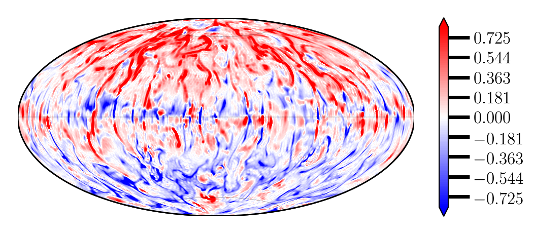
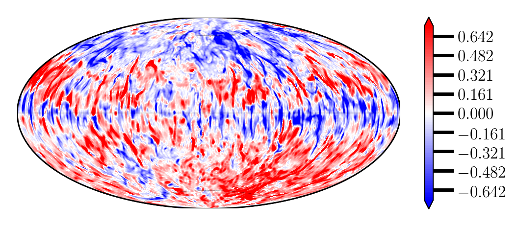
Figure 2. Result from a numerical model showing magnetic reversal. Top figure shows the normal polarity and the bottom one shows reverse polarity.
In figure 3, the angle (Θ) between the rotation axis and magnetic dipolar axis is plotted against magnetic diffusion time (td). In this figure, clear reversals and few excursions are shown. The shaded regions represent the dynamo with reversed polarity.
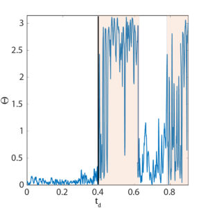
Figure 3: Dynamo axis tilting, y axis is in radian. 0 to 3.14 radian means 0 to 180 degrees.
Although the reversal has been studied by many researchers, the actual cause of reversal is a mystery. Perhaps the solution can be found by addressing the question of why rapidly rotating dynamos have a preference for dipolar solutions (Sreenivasan, 2010).
References:

J Aubert.  Geomagnetic acceleration and rapid hydromagnetic wave dynamics in advanced numerical simulations of the geodynamo. Geophys. J. Int., 214(1):531–547, 04 2018.

Bullard and H.  Gellman.   Homogeneous dynamos and terres-trial magnetism. Philos. Trans. R. Soc. A, 247:213–278, 1954.

Cattaneo D. W. Hughes. Strong-field dynamo action in rapidly rotating convection with no inertia. Phys Rev E Stat Nonlin. Soft Matter Phys, 93(6):061101, 2016.

J. Davies and D.  Gubbins. A buoyancy profile for the Earth’s core. Geophys. J. Int.,187(2):549–563, 11 2011.

Labrosse. Thermal and magnetic evolution of the earth’s core. Phys. Earth Planet. Inter.,140 (1):127 – 143, 2003.

V. R. Malkus. Magnetic field generation in electrically conducting fluids. In H. K. Moffatt. Cambridge University Press, 1978. pp 343.

A  Sheyko, C.  Finlay, and A Jackson.   Magnetic reversals from planetary dynamo waves. Nature, 539(7630):551–554, 2016.

V. Smirnov, J. A. Tarduno, and D. A. D. Evans. Evolving core conditions ca. 2 billion years ago detected  by  paleosecular  variation. Phys.Earth Planet. Inter., 187(3):225 – 231, 2011.

Sreenivasan. Modelling the geodynamo: progress and challenges. Curr. Sci., (99 (12)), 2010.

Sreenivasan, S. Sahoo, and G. Dhama. The role of buoyancy in polarity reversals of the geodynamo. Geophys. J. Int., 199(3):1698–1708, 10 2014.