
In preparation for Valentines day, Bob Myhill explores the potential for close partnership (and even love?) between the geodynamics and thermodynamics communities.
 Much of Earth and planetary science relies in some way on thermodynamics. This is not a surprise; the elegance1 of its premises makes thermodynamics a robust starting point for many investigations, and the number of thermodynamic applications across the sciences is vast. Indeed, it’s easy to believe that if eternal truth exists in scientific endeavour, it lies in thermodynamics. I’m paraphrasing Einstein there, so I’m in good company.
Geodynamics is no exception to the rule, and relies heavily on thermodynamics. Without thermodynamics, there would be no constraints on how energy depends on the local state of the system, and therefore we would have no way to solve the energy conservation equation. In compressible models, thermodynamics also provides relations between physical properties such as thermal expansivity and heat capacity. But conversely, geodynamics can provide vital constraints to petrological problems, which have traditionally been constrained only by phase equilibria.
In this blog post, I offer a brief introduction to the coupling of geodynamics and thermodynamics, and why this coupling is so valuable.
Thermodynamics and Energy Conservation
The field of geodynamics relies on the laws of conservation of mass, energy and momentum. Thermodynamics provides rules which can be incorporated into these conservation laws. Let’s take a brief look at the law of conservation of (specific internal) energy (U, J/kg) of a parcel of material (Connolly, 2009):
The contributors to the rate of change of energy in this expression are thermal diffusion, viscous/frictional dissipation, dilational work and the generation of heat by radioactivity.
In order to solve this equation, we must first understand how the state of the system affects the internal energy. Reversible changes in energy are the result of different kinds of work done on the system, which expressed in derivative form looks like this:
where -P dV represents the reversible P-V work and TdS represents the reversible heat (“thermal work”). Specific entropy2 (S) and specific volume (V = 1 / density) are therefore “natural variables”3 for specific internal energy. Energy conservation can therefore be expressed naturally in terms of entropy and density. I will explain the motivation for such a formulation later in this post, but see also Connolly (2009) for more detail.
Using this form of the energy conservation equation requires a thermodynamic dataset that provides material properties (including temperature and pressure) as a function of entropy and density. There exist several mineralogical datasets for which this is possible, and several thermodynamic programs (such as PerpleX, ENKI and BurnMan) that can process these datasets and output required information.
For those of us used to seeing phase diagrams as a function of pressure (P) and temperature (T), it can be difficult to figure out what the corresponding entropy (S) and density (ρ) diagrams might look like, and why they might be more useful to geodynamicists than their common P-T equivalents. To illustrate this, the figure below shows phase relations for Mg2SiO4 drawn using the four natural combinations of variables (T-P, S-P, T-ρ, S-ρ). The pink line on each of the plots illustrates a single isentropic path. Note that in T-P-space (top left hand diagram), the isentropic path tracks along the black univariant lines, and passes through the P-T invariant point where all four phases are stable. At the invariant point, for example, the assemblage could be composed of 100% ringwoodite, 100% periclase+bridgmanite, 100% periclase+akimotoite, or any combination of those three. Therefore, pressure, temperature and bulk composition are insufficient to uniquely determine the material properties (entropy, density etc) of the system. In S-P and T-ρ space, the P-T invariant has become a line, but there remains ambiguity over phase proportions on that line. However, in S-ρ space (bottom right), the P-T invariant point has become a divariant field (shown in purple). Thus, entropy, density and bulk composition are sufficient to uniquely determine the P-T state and the material properties of the system.
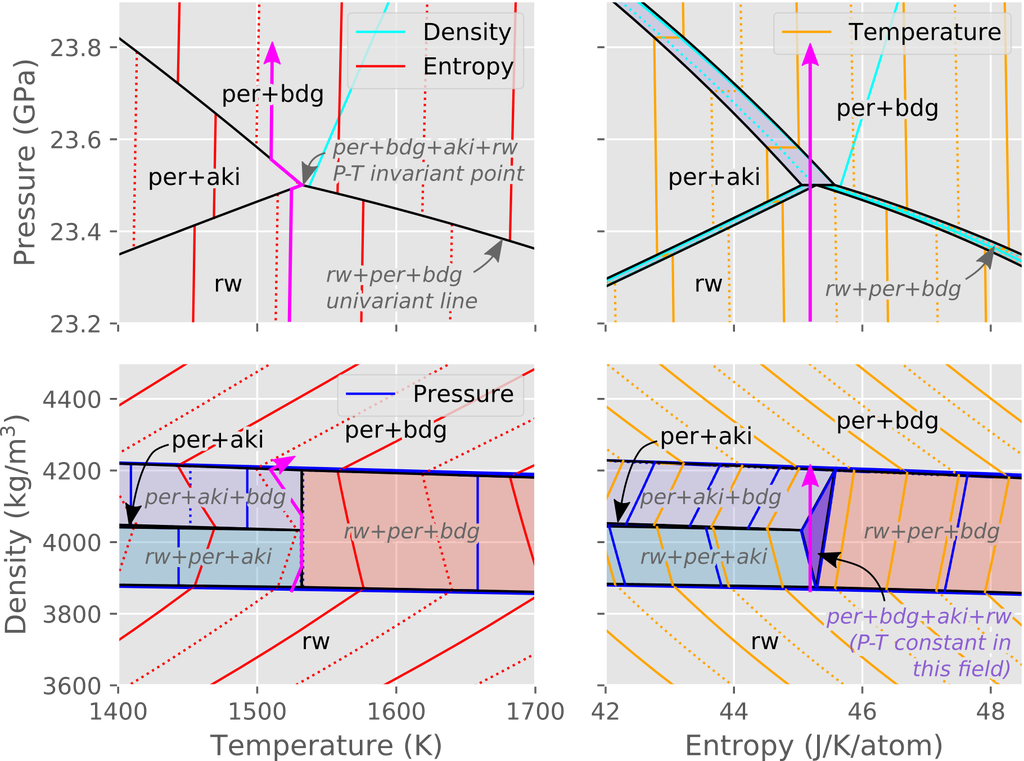
Stable mineral assemblages under upper-lower mantle boundary conditions in a forsterite (Mg2SiO4) composition. Assemblages are calculated assuming local thermobaric equilibrium. The diagrams shown are (reading left to right, top to bottom): temperature vs. pressure, entropy vs. pressure, temperature vs. density and entropy vs. density. Mineral abbreviations are as follows: ringwoodite (rw), akimotoite (aki), bridgmanite (bdg) and periclase (per). The coloured fields correspond to the univariant reaction lines in the P-T diagram. Scales and colours are consistent between diagrams. The pink arrow represents a potential isentropic path. Diagram computed using the Stixrude and Lithgow-Bertelloni (2011) database using the open-source BurnMan software (Myhill et al., 2021; Cottaar et al., 2014).
Such diagrams are also useful in and of themselves. For example, if a material is expected to take a roughly isentropic path (as is the case for a closed system), or will be subject to a fixed volume (a good approximation for a compressible inclusion in a incompressible medium) then it is much easier to visualize the succession of stability fields using entropy or density as independent variables. There are some particularly beautiful papers which highlight the insights that can be gained by such techniques (e.g. Powell et al., 2005; Stolper and Asimow, 2007).
However, the true strength of such thermodynamic analyses comes from combining them with geodynamic models. Thermal gradients and rheology can fundamentally affect the p-T-S-ρ paths taken by rocks, and interactions between deformation and reactions can potentially have a significant effect on pressure (see Moulas et al., 2013 for a review).
Effective properties in a reactive world
It may not be clear from the preceding section just what the impact of reactions is on the effective material properties that geodynamicists are used to thinking about. Why can’t we use a P-T formulation of the conservation equations with a P-T lookup table for required material properties?
Looking back at the previous figure, in P-T space the stable assemblage and associated entropy and density change discontinuously across the black univariant lines. Across these discontinuous changes the isobaric heat capacity, thermal expansivity and isothermal compressibility are all infinite:
Even in a natural mantle, where reactions often (but not always) occur across finite pressure and temperature intervals, the difference in derivative properties between the “static” unreacting assemblage and the reactive assemblage can be profound. To see why this should be the case, consider the following expression for the thermal expansivity:
The first term in the expansion represents the thermal expansivity of the static assemblage, where the amounts and compositions of the phases are not allowed to change. The second term represents the influence on the bulk properties if the different phases are allowed to react internally and with one another. A figure illustrating the difference between the static and total properties for a pyrolite composition along an isentrope is shown below. The sharp spikes in reactive properties correspond to places where the assemblage is changing rapidly (with simultaneous changes in density and entropy). The large negative spike in thermal expansivity corresponds to the narrow ringwoodite → bridgmanite + ferropericlase reaction, which has long been thought to (partially) inhibit flow between the upper and lower mantle.
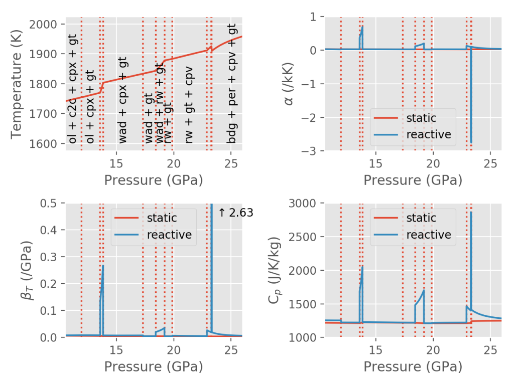
Difference between static (unreactive) and reactive properties for a model pyrolite in the system NCFMAS (Sun and McDonough, 1995) along the 1600 K isentrope, using the thermodynamic dataset of Stixrude and Lithgow-Bertelloni (2011) and the open-source BurnMan software (Myhill et al., 2021; Cottaar et al., 2014).
Thus, in P-T formulations of the conservation equation, we must deal somehow with effective properties (isobaric heat capacity, thermal expansivity and isothermal compressibility) which are both discontinuous and may vary by orders of magnitude, or may even be infinite (in the case of univariant/invariant reactions). This is commonly done by explicitly tracking the progress of reactions, but this rapidly becomes cumbersome for realistic materials. More natural S-ρ formulations have the potential to neatly avoid these problems.
Challenges and prospects for the future
This post has only touched on the coupling of geodynamics and thermodynamics in isochemical models, and I have assumed local thermobaric equilibrium throughout. I have not discussed specific implementations or extensions to chemically variable, disequilibrium systems. Progress is being made towards all of these goals (e.g. Tweed et al., 2019, Gassmöller et al., 2020, Rummel et al., 2020).
Incorporating fully consistent treatments of thermodynamics in geodynamic models is hard, so it is worthwhile to ask in which environments the coupling will have the biggest effect. Obvious places to consider are those in which relaxation of stresses/thermal diffusion is slow compared to rates of volume/entropy change. In addition to the commonly cited example of the upper-lower mantle boundary, subduction zones, and areas of strong continental crust are of particular interest (see hypotheses by Guest et al., 2004; Mancktelow, 2008 and Vrijmoed et al., 2009). And of course magmatic and hydrothermal systems are prime sites for complex geo- and thermodynamic behaviour (e.g. Norton and Dutrow, 2001).
These are particularly exciting times for the coupling between geodynamics and thermodynamics, and I can’t wait to see what new discoveries lie around the corner.
- I had originally written “simplicity” here, because that’s the word that Einstein used. But thermodynamics is a field riddled with missteps and misconceptions (Truesdell, 1980), and many papers and even some textbooks are entirely opaque.
- Circa 1000-word blog posts could never do justice to the gnarly concepts of entropy and temperature. Thankfully there are many excellent works on the subject, including the classic textbooks by Fast (1970) and Blundell and Blundell (2012), and exceptionally clear papers by E.T. Jaynes (including the collection edited by Rosenkrantz, 2012).
- Natural variables are variables with which thermodynamic potentials (internal energy, enthalpy etc.) can be differentiated to yield all other thermodynamic properties of the system.
References
Blundell, S.J. and Blundell, K.M., 2009. Concepts in thermal physics. OUP Oxford.

Connolly, J.A.D., 2009. The geodynamic equation of state: what and how. Geochemistry, Geophysics, Geosystems, 10(10).

Cottaar, S., Heister, T., Rose, I., and Unterborn, C:
BurnMan – a lower mantle mineral physics toolkit
Geochemistry, Geophysics, Geosystems 15.4 (2014): 1164-1179.

Fast, J.D., 1970. Entropy. Macmillan International Higher Education.

Gassmöller, R., Dannberg, J., Bangerth, W., Heister, T. and Myhill, R., 2020. On formulations of compressible mantle convection. Geophysical Journal International, 221(2), pp.1264-1280.

Guest, A., Schubert, G. and Gable, C.W., 2004. Stresses along the metastable wedge of olivine in a subducting slab: possible explanation for the Tonga double seismic layer. Physics of the Earth and Planetary Interiors, 141(4), pp.253-267.

Mancktelow, N.S., 2008. Tectonic pressure: Theoretical concepts and modelled examples. Lithos, 103(1-2), pp.149-177.

Moulas, E., Podladchikov, Y.Y., Aranovich, L.Y. and Kostopoulos, D., 2013. The problem of depth in geology: When pressure does not translate into depth. Petrology, 21(6), pp.527-538.

Myhill, R., Cottaar, S., Heister, T., Rose, I., and Unterborn, C. (2021):
BurnMan [Software]. Computational Infrastructure for Geodynamics. https://github.com/geodynamics/burnman/

Norton, D.L. and Dutrow, B.L., 2001. Complex behavior of magma-hydrothermal processes: role of supercritical fluid. Geochimica et Cosmochimica Acta, 65(21), pp.4009-4017.

Powell, R., Guiraud, M. and White, R.W., 2005. Truth and beauty in metamorphic phase-equilibria: conjugate variables and phase diagrams. The Canadian Mineralogist, 43(1), pp.21-33.

Rosenkrantz, R.D. ed., 2012. ET Jaynes: Papers on probability, statistics and statistical physics (Vol. 158). Springer Science & Business Media.

Rummel, L., Baumann, T.S. and Kaus, B.J., 2020. An autonomous petrological database for geodynamic simulations of magmatic systems. Geophysical Journal International, 223(3), pp.1820-1836.

Stixrude, L. and Lithgow-Bertelloni, C., 2011. Thermodynamics of mantle minerals-II. Phase equilibria. Geophysical Journal International, 184(3), pp.1180-1213.

Stolper, E. and Asimow, P., 2007. Insights into mantle melting from graphical analysis of one-component systems. American Journal of Science, 307(8), pp.1051-1139.

Truesdell, C., 2013. The tragicomical history of thermodynamics, 1822–1854 (Vol. 4). Springer Science & Business Media.

Tweed, L.E., Spiegelman, M.W., Kelemen, P.B., Ghiorso, M.S., Evans, O. and Wolf, A.S., 2019. A Tractable Approach to Coupling the Thermodynamics, Kinetics, and Fluid Dynamics of Mantle Melting. AGUFM, 2019, pp.V21B-02.

Vrijmoed, J.C., Podladchikov, Y.Y., Andersen, T.B. and Hartz, E.H., 2009. An alternative model for ultra-high pressure in the Svartberget Fe-Ti garnet-peridotite, Western Gneiss Region, Norway. European Journal of Mineralogy, 21(6), pp.1119-1133.