The huge amount of data produced in Geosciences is increasing exponentially, and numerical modelling has become a key tool for understanding tectonic evolution over time, which also increases the volume of data produced. Here, I, João Bueno (PhD student at University of São Paulo, Brazil) will present how a machine learning technique known as Self-Organising Maps can be used to understand the interaction between variables and their evolution in numerical models. This technique has been applied in many fields, such as finance, climate and geography, with great results when investigating high-dimensional datasets. It has enormous potential for use in tectonic studies.
Large datasets, huge challenges!
Geodynamic modelling often produces many results and datasets, making the modelling analysis a challenging task for geoscientists. It is very common to have enormous datasets, with tens of gigabytes and many variables for the mesh nodes or elements. These can include scalar variables (like temperature, viscosity, and strain), vectorial variables (heat flux and/or velocity), and even tensors (such as stress). Furthermore, it is common not only to investigate one variable at one time step, but also its interactions with the other variables and how it evolves over time.

João Paulo de Souza Bueno is a Brazilian PhD student researching salt tectonics and the thermal blanket effect, with a particular focus on how it can alter the topography and temperature field of rifted margins using geodynamic models.
This volume of data represents just one scenario; in practice, dozens of scenarios are often analysed. The comparison between geodynamic scenarios and tectonic settings is often complex and is strongly influenced by our expertise in geology, geophysics and numerical methods. After personally struggling with these problems during my research, I watched a great presentation about Self-Organizing Maps (SOM) by Professor Cleyton Carneiro, from the University of São Paulo, suggesting a possible solution. His research team had compiled around 20 spatial variables in an attempt to classify remote sensing images, achieving amazing results.
In a nutshell, Self-Organizing Maps are a topological neural network that learns a certain data pattern and creates a 2D representation or “map” view from the original variables. Since a geodynamic simulation can be considered as “spatial variables” over time, it is intuitive to consider that machine learning techniques can be used to examine large datasets from these kinds of models. This was exactly what we did with the help of Profs. Cleyton Carneiro and Rafael Gioria (both from POLI-USP in Brazil). With this approach, it was possible to train a SOM neural network using intraSOM library (De Gouvêa et al., 2023) to visualise tendencies and to observe how the neurons “learned” what was happening in the modelled materials.
How do these “Maps” work?
Self-Organizing Maps are an effective tool to visualise and to compile high-dimensional data, allowing the visualization of n-dimensions on 2D projections (Kohonen, 1998). An initial neural network is trained using a dataset, in which a neural network will learn how to represent the data. In SOM, the neurons are represented as graphs, with a topological arrangement that can deform in learning iterations (Figure 1). A common initial grid setting is the hexagonal, where each neuron has six neighbouring neurons, but a regular four neighbours is also possible. To avoid edge effects on the maps, we can use a toroidal topology on neuron’s network, creating a ‘doughnut’ shape instead of a planar map. This ensures that a neuron at the top edge is directly connected to one at the bottom, creating a continuous surface (Mount & Weaver, 2011).
After dataset pre-processing and the neural network initialisation, the training process consists of two main phases. The first is the competitive phase, where neurons compete to find the one that best represents a sample. The neuron with the smallest distance to the sample is declared the Best-Matching Unit (BMU). The following stage is the cooperative phase, where the BMU influences the network to improve the fit to the samples. In this phase, the neighbouring neurons are pulled towards the BMU, making the topological structure behave like an elastic net (Figure 1). This mechanism drives the learning process, as the BMU and its neighbours adjust their weights to match the input patterns.
Figure 1: Example of neuron training in a SOM algorithm in a rectangular grid on a 2D-dataset. This network has a planar topology with a rectangular 4-neighbour grid. Image from the Wikimedia.
There are two primary methods to visualise the trained map: component plots and U-Matrices. Component plots visualise the weight distribution of each variable across the lattice, allowing for the identification of correlations by comparing different variables. Conversely, an U-Matrix is essential for detecting “natural classes” (Figure 2). It represents the average Euclidean distance between adjacent neurons, where high values act as topological “walls” separating clusters, while low values indicate high similarity within a domain.
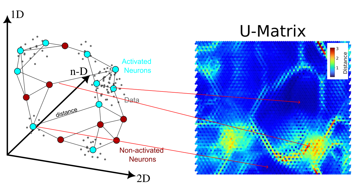
Figure 2: Example of how a trained neural network is plotted in the U-matrix plot (credit: author).
Training a neural network with geodynamic models
We tested the efficacy of the SOM on a modelled rift system. For simplicity, the neurons were trained using a wet-quartizite crust scenario, with a 3 km thick layer of pre-rift sediment, where the lithosphere is stretching at a velocity of 2 cm/y. The Mandyoc code (Sacek et al., 2022) was used, considering a 1200×300 km finite element grid with 1×1 km resolution. In this scenario, the first shear zone developed after ~5.5 Myr, mantle breakup occurred after 8.2 Myr, and crust breakup occurred after ~13 Myr (Figure 3).
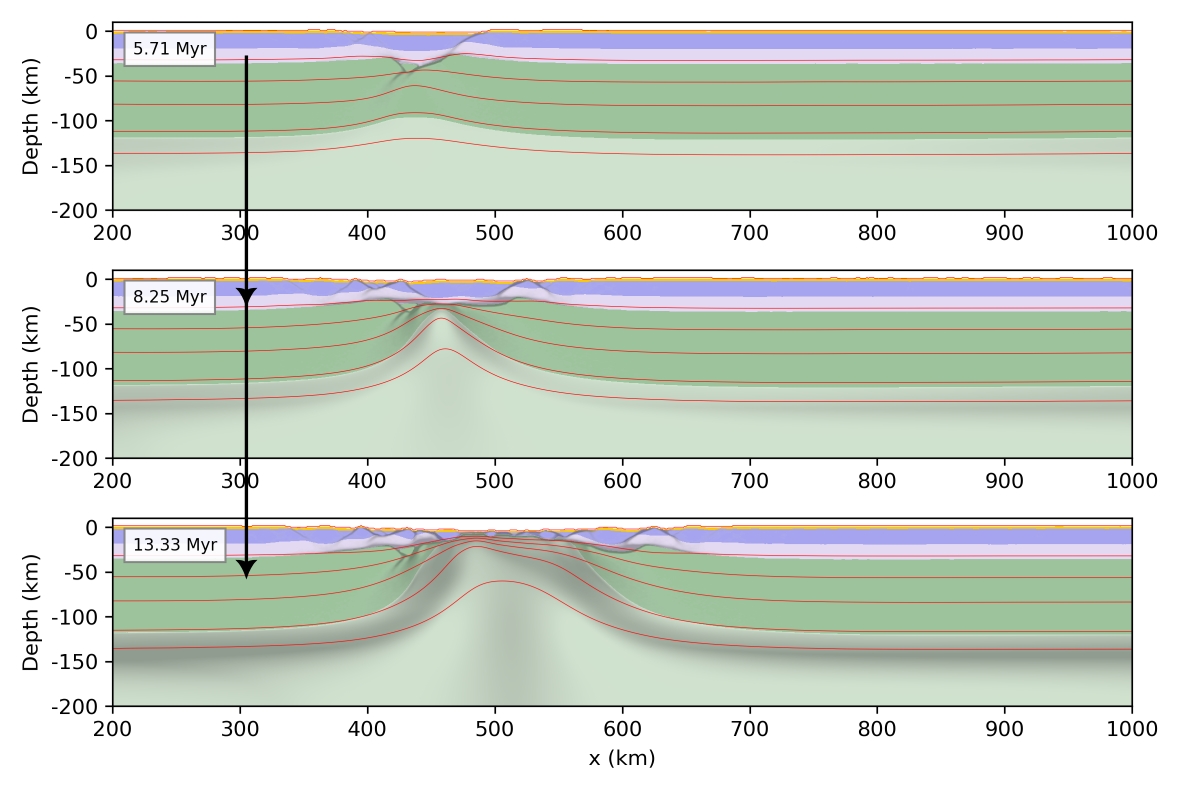
Figure 3: Evolution of the rift system model over time. Isotherms are from 600 to 1200 °C in lithosphere (credit: author).
The temperature, viscosity, strain, strain rate, density and deviatoric horizontal stress were pre-processed and filtered in order to train a first self-organizing map, which had a hexagonal topology (where each neuron has six neighbours) and toroidal geometry. These variables were chosen because they are closely related to the state of the crust. High strain rates can be common in many materials; however, when coupled with high temperatures, they specifically indicate ductile deformation. Only the crustal elements at the 3 mentioned timesteps (Figure 3) were used. As the training of the neurons was successful, we can plot and observe what each neuron learned, and compare “regimes” within our input (Figure 4).
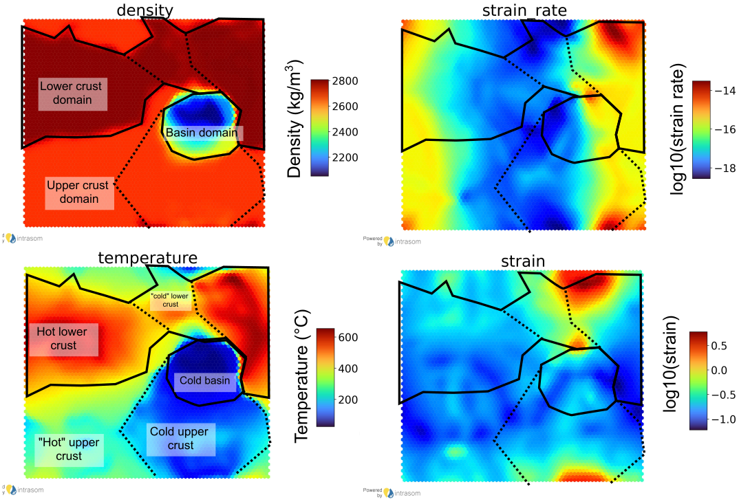
Figure 4: Component plots for some trained variables. Each plotted cell (hexagon) represents a neuron, and the colour indicates the value that the neuron represents for that feature. The dashed line separates the temperature zones, and the solid line separates the material’s domain. Please note that the x- and y-axis have no real meaning in this plot. The present figures and results were made by the intraSOM library (De Gouvêa et al., 2023). IntraSOM is a fully Python-based implementation of self-organizing maps (SOM) developed by the Integrated Technology for Rock and Fluid Analysis (InTRA) research center of the University of São Paulo and is available on GitHub. (credit: author).
Using the relationship between density and the temperature, we were able to trace the material domains (solid lines) and the temperature zones (dashed lines). As expected, the high strain rates are predominant in high temperature zones (ductile deformation), while limited strain rates in low-temperature zones are related to brittle deformation, which only occurs in the basin and upper crust. Regions with very low strain rates are not undergoing deformation, probably because they represent the model boundaries. The strain also indicates significant deformation of the lower crust due to stretching. However, intermediate strain can occur in all materials and temperatures, corresponding to faulted rocks in cold zones and weakened materials in hot zones.
This basic geological interpretation was possible by considering just these few variables! More complex models with additional features can provide further insights, offering a more comprehensive view of the entire context. It is also possible to merge data, handle missing data and apply this technique in many contexts within the geosciences (Bação et al., 2005; Klose, 2006). Taken together, this shows how versatile and valuable this technique can be for understanding complex geodynamic systems.
References

Bação, F., Lobo, V., & Painho, M. (2005). The self-organizing map, the Geo-SOM, and relevant variants for geosciences. Computers & Geosciences, 31(2), 155–163. https://doi.org/10.1016/j.cageo.2004.06.013

De Gouvêa, R. C. T., Gioria, R. D. S., Marques, G. R., & Carneiro, C. D. C. (2023). IntraSOM: A comprehensive Python library for Self-Organizing Maps with hexagonal toroidal maps training and missing data handling. Software Impacts, 17, 100570. https://doi.org/10.1016/j.simpa.2023.100570

File:TrainSOM.gif. (2025, November 2). Wikimedia Commons. Retrieved January 16, 2026, from https://commons.wikimedia.org/w/index.php?title=File:TrainSOM.gif&oldid=1107782967.

inTRA-USP, IntraSOM, GitHub Repository, https://github.com/InTRA-USP/IntraSOM.

Mount, N.J., Weaver, D.  (2011). Self-organizing maps and boundary effects: quantifying the benefits of torus wrapping for mapping SOM trajectories. Pattern Analysis and Applications, 14, 139–148. https://doi.org/10.1007/s10044-011-0210-5

Klose, C. D. (2006). Self-organizing maps for geoscientific data analysis: Geological interpretation of multidimensional geophysical data. Computational Geosciences, 10(3), 265–277. https://doi.org/10.1007/s10596-006-9022-x

Kohonen, T. (1998). The self-organizing map. Neurocomputing, 21(1–3), 1–6. https://doi.org/10.1016/S0925-2312(98)00030-7

Sacek, V., Assunção, J., Pesce, A., & Da Silva, R. M. (2022). Mandyoc: A finite element code to simulate thermochemical convection in parallel. Journal of Open Source Software, 7(71), 4070. https://doi.org/10.21105/joss.04070
