It is common to hear that a good illustration is better than a lengthy textual explanation, and we fully agree with that statement.
We are used to retrieving information and understanding things through visual illustrations. In the scientific community, any paper comes with a number of plots to show the data, and diagrams to explain concepts, ideas or workflows. For example, a typical plot that hydrologists would produce to show the hydrological regime of a catchment is a bar chart with the interannual average of streamflow for each month. Although it is highly summarized, it gives a very quick and broad idea of the type of hydrological regime at play.
However, we are so used to communicating information through visual means that we tend to forget about other ways. Indeed, why not use another one of our senses? Why not use our hearing capabilities? Could not sounds, or even music (i.e. sounds organized in a nice-to-hear way) be a relevant and efficient way to communicate science?
Exploring data sonification in hydrology
It turns out that using sound to communicate information contained in data is not new. It is called data sonification. There is even “The Sonification Handbook”, written by Thomas Hermann, Andy Hunt and John G. Neuhoff, published in 2011, where the subject is thoroughly dealt with. Because a 500+ pages long handbook may be a little overwhelming, here are three eloquent examples:
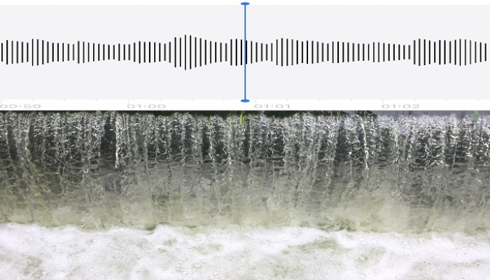
- Earthquake example: here the seismic signal is directly interpreted as a sound wave; it is the most straightforward way to use sound to communicate data.
- Asteroid impact example: here, a synthetic sound is emitted each time an asteroid hits the moon; it is an event-based sonification that aims at emphasizing when and how often an event of a certain type occurs.
- Temperature example: here the temperature series of one region is mapped to the pitch of one instrument; this is an example of what is called parameter mapping.
This blog post will focus on the technique featured in the last example: parameter mapping.
Parameter mapping is the action of mapping some data (e.g. streamflow or precipitation time series at the outlet of a catchment) to an attribute of notes (e.g. the pitch, the volume, the panning).
We built a web application, called Hydrological Soundscapes, where you can see and, more importantly, hear hydrological regimes from all around the world!
The Hydrological Soundscapes App
We explain below how this app was built providing a concrete example of data sonification in hydrology.
But before reading further, we invite you to first check out the app (with a good headset!) and see… or rather hear for yourself.

General approach used to build Hydrological Soundscapes
About the data
We used a selection of 1420 hydrometric stations from the worldwide dataset GSIM. For each station, the streamflow time series was used to compute four variables frequently used in hydrology to summarize average, high and low flows: the interannual average flow, the 12 monthly interannual flows, the fraction of annual maxima falling in each of the 12 months, and similarly the fraction of annual minima of 30-day flows falling in each month. In the end, each hydrometric station was associated with three times 12 values plus the interannual flow (see the example figure below).
The last (secret) ingredients used in the app are the coefficient of variations associated with the monthly variables (more on this later).

For each hydrometric station, four hydrological variables are used in Hydrological Soundscapes
About the sounds
We used three different instruments: a piano, a bass and a hang drum.
Recorded sound samples (one sample per note) were used rather than synthetic sounds since they are generally much nicer to listen to.
The choice of instruments was guided by the need to clearly identify each instrument when they’re all playing together. Instruments with different pitch ranges (low for the bass, average for the piano and high for the hang drum) and different natures of sound were thus chosen.
Finally, regarding the note attributes considered in the parameter mapping, we limited ourselves to pitch and volume. A last musical attribute (as opposed to note attribute) was considered: the tempo.
About the mapping between data and sound
Then comes the mapping part that glues everything together.
Average monthly streamflow data was associated with the piano since the piano plays in the average pitch range and can be considered as the lead instrument in our formation. We chose to map the seasonality of annual maxima to the bass and the seasonality of annual minima to the hang-drum. These choices are subjective: it seemed to us that hang-drum sounds are more evocative of drought conditions, while bass sounds are more fitted to floods, but you may disagree with this!
Deciding which instrument should be associated with which variable is only the first step. The mapping itself is performed on the pitch and the volume of the notes. For the pitch, musical scales were used ensuring that the resulting sounds would remain in harmony, at the expense of discretizing the hydrological variable. The volume of each note was set to be inversely proportional to the coefficient of variation of each monthly variable: this allows “fading out” months for which the interannual value hides a large variability, while creating a dynamic musical phrasing.
Finally, the tempo is controlled by the interannual average streamflow.
Interesting questions arose from this mapping process. For example, should larger streamflow values be mapped to higher pitch or lower pitch? In the app we offer the possibility to invert the mapping of the piano to explore how this choice affects perception. Making such music-related decisions to make sonification sounds good was the most time consuming but also the most interesting, fun, subjective and even artistic part of building Hydrological Soundscapes. Quite some time was spent experimenting and we quickly realized that it could be endless. Some choices are left open in the app so that the user can experiment.
Why mapping hydrological data as sound variables
Hydrological Soundscapes has multiple ambitions. It aims at being informative (differences in hydrological regimes can be heard by comparing different parts of the world). We also tried to make it interactive and playful (it is fun and even addictive – we speak for ourselves anyway – to play with the different options offered by the app). Finally, we wanted the result to be nice to hear (the sounds created although far from a musical piece are still nice to the ear).
Therefore, we believe that such an app can engage a broad audience and have an interest beyond the hydrological community.
We hope this example of data sonification ignited your curiosity and made you not see but hear hydrological regimes in a different way.
For more examples of data sonification in the hydrologic context, you may consult here.
If you want to experiment yourself with data sonification, here are a few useful resources:
- Github repository of Hydrological Soundscapes
- Github repository of the content of globxblog blog
- Some preliminary R packages: here and here.
- A web application to sonify your own data
We probably missed some relevant examples of data sonification related to hydrology so we encourage you to share other applications with us in the comment section!
Edited by Maria-Helena Ramos
Pingback: Cryospheric Sciences | Perspective on Listening to Permafrost