Could our present day “warm” climate turn into a frozen fully glaciated one, as if the whole Earth is a huge “snowball”? That was a question put forward independently by Mikhail Budyko and William Sellers in the late 60s [1,2] who made a first estimate of the necessary changes of incoming solar radiation, such that either the Arctic ice sheet completely melts, or the planet gets fully frozen. Based on the ice-albedo feedback mechanism, and viewing the climate as a simplified thermodynamical system, they used Energy Balance Models (EBM) to predict that both scenarios can occur for a roughly ±2-5% change, respectively. Such EBMs can effectively characterize, within different levels of complexity, the interplay between the incoming and outgoing solar radiation with simplified/parameterized internal elements of the climate system (e.g., ocean, atmosphere) [3]. Note that the elementary principles of EBMs are at the core of modern state of the art climate models [4].
These studies [1-3], and the discussion they later sparked in the 70s-80s [5] hinted a quantification of risk for an abrupt climate change due to a sudden nuclear winter, caused by a full-scale nuclear war, or even a large asteroid impact or super-volcano eruption. The idea is simple: such catastrophic events would quickly unleash smog and particulate matter into the atmosphere, covering it from sunlight. In such conditions, if solar radiation cannot reach the Earth’s surface persistently for a few years, then the global temperature will quickly drop. The problem is that even when the sky eventually clears out, if the ground is fully frozen, and sea-ice has developed beyond a critical latitudinal extent, the system cannot return to the warm climate, because the snowball earth is a stable climate. Given the current astronomical configuration, the Earth can exhibit at least two stable climate states, the warm and the snowball; see in Fig. 1 the bifurcation diagram from the EBM used in [3,10], where in red is the Warm branch, in blue the Snowball and in green the unstable branch, versus the non-dimensional parameter μ=S/S0, with S0=1365W/m2. In realistic conditions, transitioning from one state to the other is quite hard and rare. Paleoclimatology studies reveal that the Earth has indeed suffered at least two global glaciations in the past, namely 630 and 715 million years ago, and many less severe ice-ages [6-8].
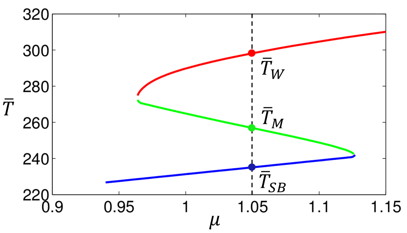
Fig. 1. Bifurcation diagram of the average temperature versus the non-dimensional Solar irradiance μ. Adapted from [10].
Building upon [1-3] and with tools from Dynamical systems theory, together with modern climate models, it is possible to not only reconstruct and study the snowball climate state, but also to explore a rich “world” of possible climate states. This viewpoint was recently put forward by Valerio Lucarini and collaborators, where at given physical parameters, the possible climate states can be seen as lying on a high-dimensional dynamical landscape. This allows to unfold the multiscale and multistable nature of one of the most complex physical systems, a planetary climate [4]. By multiscale we identify how climatic characteristics and elements (e.g. rainforests, deserts, circulation patterns, etc.) extend in a multitude of spatial scales. By multistable we describe how stable such climatic characteristics and elements are with respect to temporal scales. More interestingly, this allows for their hierarchical categorization based on their spatial extent and stability properties; see Fig. 2 where one moves from level 1 to 3.
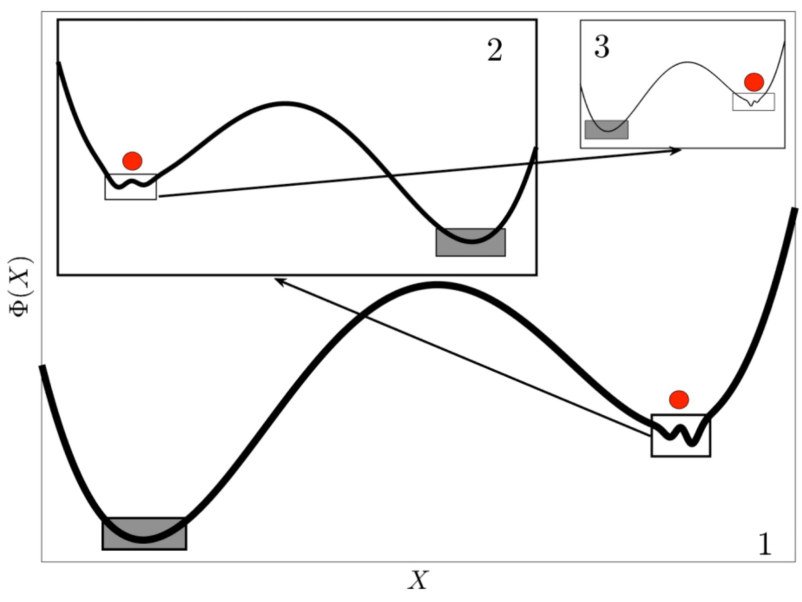
Fig. 2. Schematic representation of the multiscale nature of multistability in a climate system. Φ is the coarse-grained landscape and X a variable of the system. From [14].
In the late 70s, Klaus Hasselmann [9], using arguments of time-scale separation, proposed the idea of describing the impact of fast weather variables (atmosphere) on slower climatic variables (oceanic, cryosphere, land vegetation etc.) via stochastic perturbations modulated by Gaussian noise; therefore, enhancing climate variability, which was vital for earlier climate models. In the context of Fig. 2, by introducing some form of appropriately defined noise into the system, it is possible to explore the different levels of hierarchy of the underlying dynamical landscape. For instance, in a series of works [10-14] Gaussian perturbations are introduced to the present-day mean of solar irradiance S0 to trigger global transitions between the warm and snowball state in several climate models, ranging from a simple EBM to intermediate complexity climate models with ocean and sea-ice dynamics. This approach not only quantifies the most probable transition paths in this landscape but can also provide an evaluation of the transition probability at a given noise amplitude, as it can estimate the values of the generalized energy barriers that separate the competing stable states. In [14] the authors applied a data-driven manifold learning method to classify regions of stability within the dynamical landscape and even locate a metastable third climate state, colder than our present day warm, but with an ice-free latitudinal band.
Finally, there is a further freedom in the type of the chosen noise, as a noise different than Gaussian can be applied. In a recent preprint [15] the authors chose a Lévy type of noise which is different from Gaussian in the sense that the system can exhibit strong “kicks”. They applied it to an EBM like [3,10] and concluded that transition paths and probabilities will be different when choosing a Gaussian versus a Lévy type of noise. This is seen in Fig. 3, where a 2D coarse-grained projection of the phase space can be obtained by measuring the joint probability density function (PDF) of the system’s evolution considering the globally averaged surface temperature T versus the Equator minus Poles temperature difference ΔΤ. The deterministic attractors are given by the colored points, where red-warm, blue-snowball, green-unstable, and the averaged paths in blue and red. Notice that, sudden and dramatic events, such as massive nuclear war, a large asteroid impact or a super-volcano eruption, mentioned before, could be seen as “kick” events, and therefore well described by a Lévy type of noise. Combining the two types of noise in the same process is also possible. A promising expectation for future directions would be to quantify transition probabilities in local and multistable climatic elements and assess the risk of the associated tipping points [16].
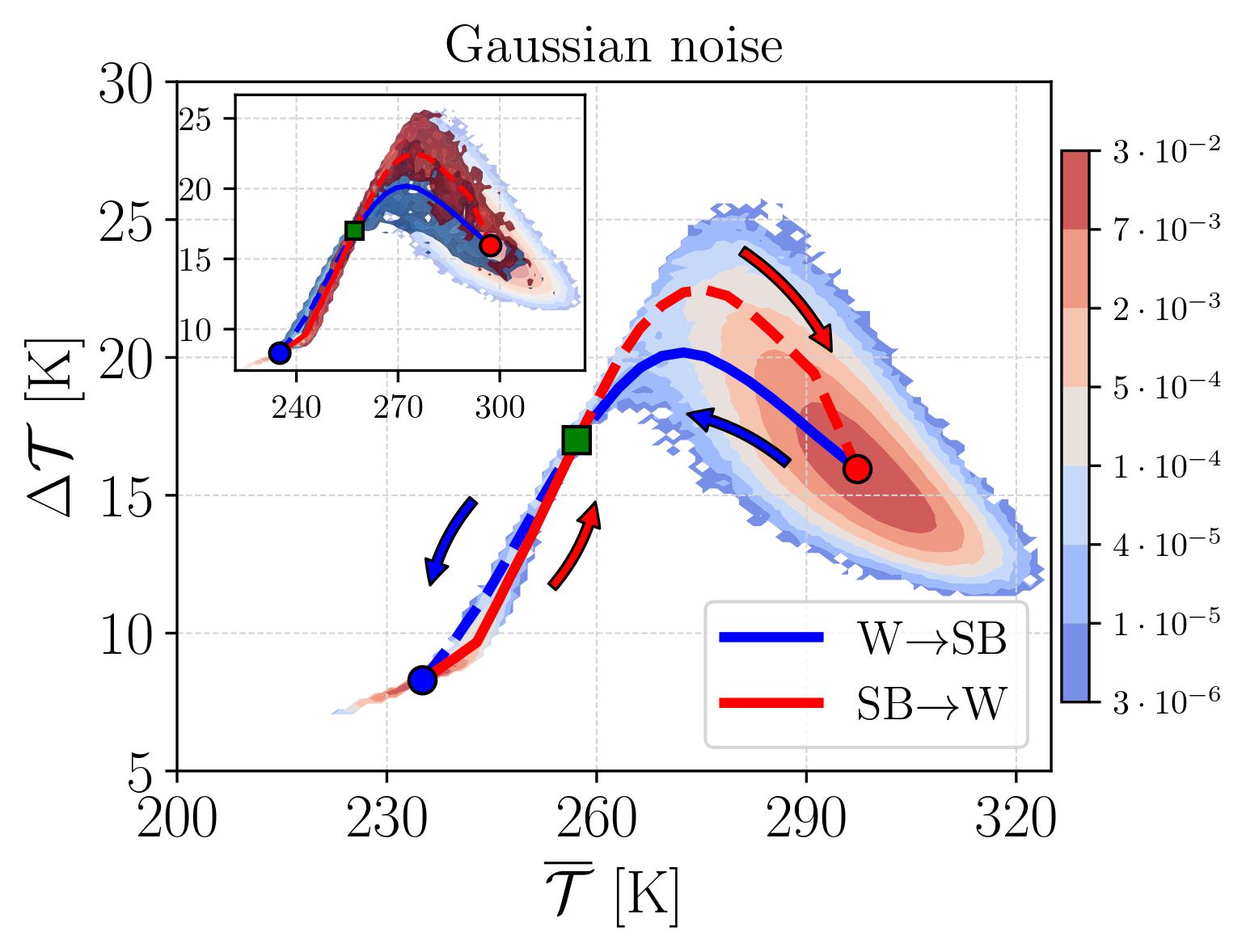
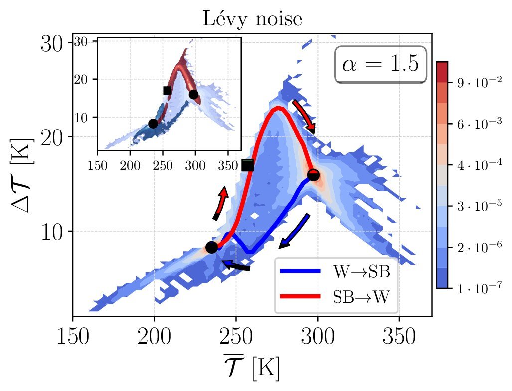
Fig. 3. Joint PDF of global temperature T versus Equator minus poles temperature difference ΔΤ for (upper) Gaussian and (lower) Lévy noise. The arrows show the direction of the most probable transition paths and the inset gives the “cloud” of transitions. From [15].
References
1. Budyko MI. 1969 The effect of solar radiation variations on the climate of the Earth. Tellus 21, 611–619. https://doi.org/10.3402/tellusa.v21i5.10109
2. Sellers WD. 1969 A global climatic model based on the energy balance of the earth-atmosphere system. J. Appl. Meteorol. 8, 392–400. https://journals.ametsoc.org/view/journals/apme/8/3/1520-0450_1969_008_0392_agcmbo_2_0_co_2.xml
3. Ghil M. 1976 Climate stability for a Sellers-type model. J. Atmos. Sci. 33, 3–20. https://journals.ametsoc.org/view/journals/atsc/33/1/1520-0469_1976_033_0003_csfast_2_0_co_2.xml
4. Ghil M, Lucarini V. 2020 The physics of climate variability and climate change. Rev. Mod. Phys. 92, 035002. https://doi.org/10.1103/RevModPhys.92.035002
5. Oldfield, J.D. (2016), Mikhail Budyko’s (1920–2001) contributions to Global Climate Science: from heat balances to climate change and global ecology. WIREs Clim Change, 7: 682-692. https://doi.org/10.1002/wcc.412
6. Pierrehumbert R, Abbot D, Voigt A, Koll D. 2011 Climate of the neoproterozoic. Annu. Rev. Earth Planet Sci. 39, 417–460. https://doi.org/10.1146/annurev-earth-040809-152447
7. Hoffman PF, Kaufman AJ, Halverson GP, Schrag DP. 1998 A neoproterozoic snowball earth. Science 281, 1342–1346. https://doi.org/10.1126/science.281.5381.1342
8. Hoffman, PF., et al. “Snowball Earth climate dynamics and Cryogenian geology-geobiology.” Science Advances 3.11 (2017): e1600983. https://doi.org/10.1126/sciadv.1600983
9. K. Hasselmann (1976) Stochastic climate models Part I. Theory, Tellus, 28:6, 473-485, https://doi.org/10.3402/tellusa.v28i6.11316
10. Bódai T, Lucarini V, Lunkeit F, Boschi R. 2015 Global instability in the Ghil–Sellers model. Clim. Dyn. 44, 3361–3381. https://doi.org/10.1007/s00382-014-2206-5
11. Lucarini V, Bódai T. 2017 Edge states in the climate system: exploring global instabilities and critical transitions. Nonlinearity 30, R32–R66. https://doi.org/10.1088/1361-6544/aa6b11
12. Lucarini V, Bódai T. 2019 Transitions across melancholia states in a climate model: reconciling the deterministic and stochastic points of view. Phys. Rev. Lett. 122, 158701. https://doi.org/10.1103/PhysRevLett.122.158701
13. Lucarini V, Bódai T. 2020 Global stability properties of the climate: melancholia states, invariant measures, and phase transitions. Nonlinearity 33, R59–R92. https://doi.org/10.1088/1361-6544/ab86cc
14. Margazoglou, G., Grafke, T., Laio, A., and Lucarini, V.: Dynamical landscape and multistability of a climate model, Proceedings of the Royal Society A: Mathematical, Physical and Engineering Sciences, 477, 20210 019, https://doi.org/10.1098/rspa.2021.0019, 2021.
15. Lucarini, V., Serdukova, L., and Margazoglou, G.: Lévy-noise versus Gaussian-noise-induced Transitions in the Ghil-Sellers Energy Balance Model, Nonlin. Processes Geophys. Discuss. [preprint], https://doi.org/10.5194/npg-2021-34, in review, 2021.
16. Lenton, TM., et al. “Climate tipping points—too risky to bet against.” (2019): 592-595. https://doi.org/10.1038/d41586-019-03595-0