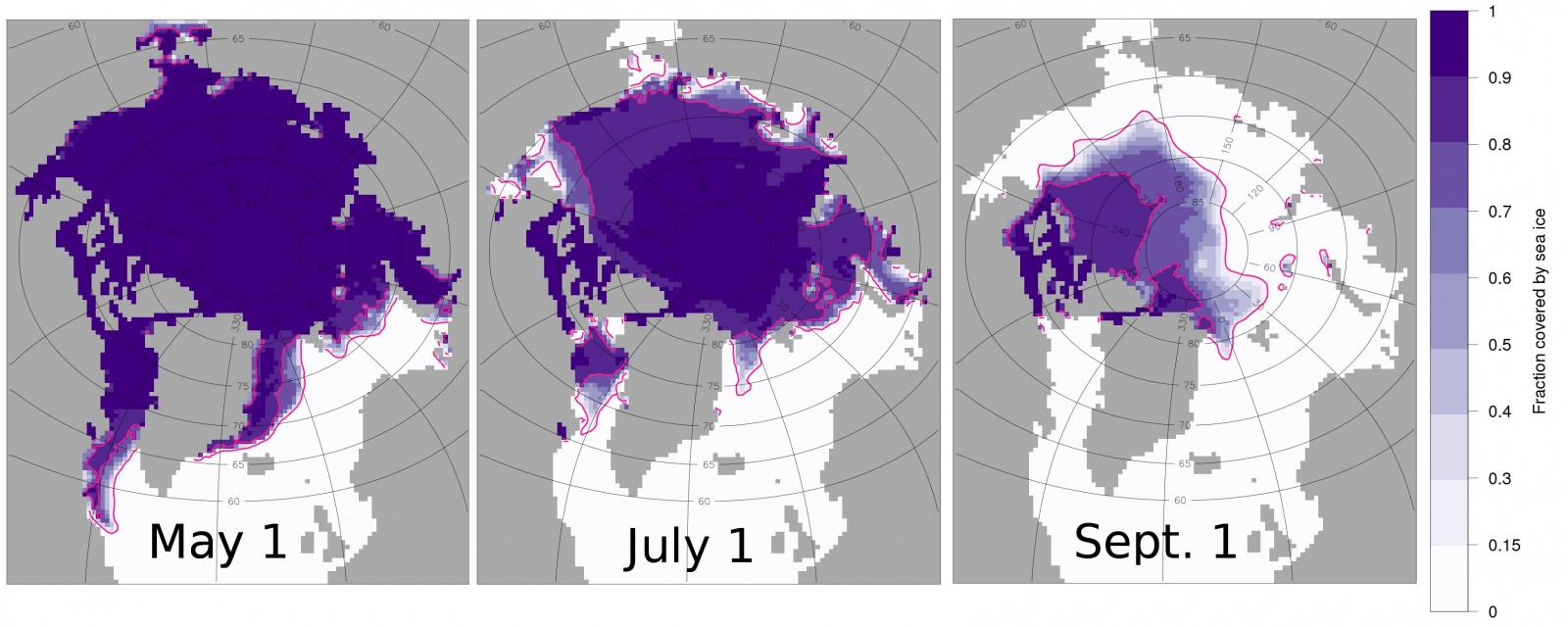
Figure 1: Sea ice extent in 2014 during the melting season. The pink lines mark the inner and outer extent of the marginal ice zone. The data comes from the CPOM setup of the CICE sea-ice model run with 9 years spin up from 2005. [Credit: Adam Bateson]
The Marginal Ice Zone
As both atmospheric and ocean average temperatures increase over the 21st century, the region of the Arctic considered either marginal or seasonal i.e. regions where sea ice is present for at least some of the year but with periods of either no or incomplete sea ice cover, is projected to increase significantly. Our image of the Week (Fig. 1) shows how the Marginal Ice Zone (defined here as regions with 15 % – 80 % ice coverage) evolves through the melting season. This means that the thermodynamic (i.e. melting, freezing) and dynamic (i.e. mechanical) processes which dominate the marginal ice zone are likely to become more important in influencing how the sea ice evolves in future.
Floe size matters
A key parameter to describe the behaviour of this region is the size of the individual ice floes – sheets of floating sea ice – which form the sea ice cover (see also a previous post on this topic). Floe size impacts melt rate, floe mechanical response, atmosphere-ocean momentum exchange and wave-ice interactions (Fig. 2). The sea ice component of climate models usually assumes all floes have the same, constant size; this assumption removes the ability of sea ice models to represent the complexity of the marginal ice zone. As a result processes which influence floe size such as wave induced break up of floes and lateral melting can’t be represented adequately in current climate models.
Figure 2: Video shows significant wave height in 2014 (darker blue colours indicate bigger waves; note also that a white colour indicates no waves, not necessarily sea ice cover). The purple/pink lines mark the inner and outer extent of the Marginal Ice Zone respectively. The data come from the CPOM setup of the CICE sea-ice model run with 9 years spin up from 2005. [Credit: Adam Bateson]
How can we represent different floe sizes in models?
Given the changing Arctic environment, representing floe size as a variable quantity is likely to be important for future accuracy of sea ice modelling. Currently sea ice models tend to divide the Polar Regions into grid cells, with properties defined as an average across the grid cell. However floe sizes can vary significantly over sub kilometre scales. There are four alternative approaches to representing such a non-uniform distribution of floe sizes within a grid cell:
- Define floes individually within the model and allow each floe to evolve independently.
- Use a categorical floe size distribution i.e. assign floes to size categories of 1 – 10 m, 10 – 20 m etc. (e.g. Horvat et. al, 2015).
- Impose a floe size distribution on each grid cell which evolves over time driven by relevant processes such as lateral melting or floe break-up (e.g. Williams et. al, 2013 a & b).
- A single floe size for each grid cell is diagnosed from the fractional ice coverage.
Option 1 would be the ideal approach from a Physics perspective. It assumes nothing about what form the floe size distribution may take and allows us to properly assess the impact of different processes for floes of different sizes. This approach is computationally expensive however, which means it will take longer for models to run. Option 4 would the simplest option and wouldn’t have negligible impacts on model run times, however it wouldn’t be possible to include in the model any processes which influence floe size. Option 2 and option 3 represent intermediates between these two extremes. In particular option 3 would be a preferred compromise if floes can be represented as a coherent distribution which evolves over time at the grid length scale.
We should now look at whether observations support the use of such a distribution.
The power law distribution
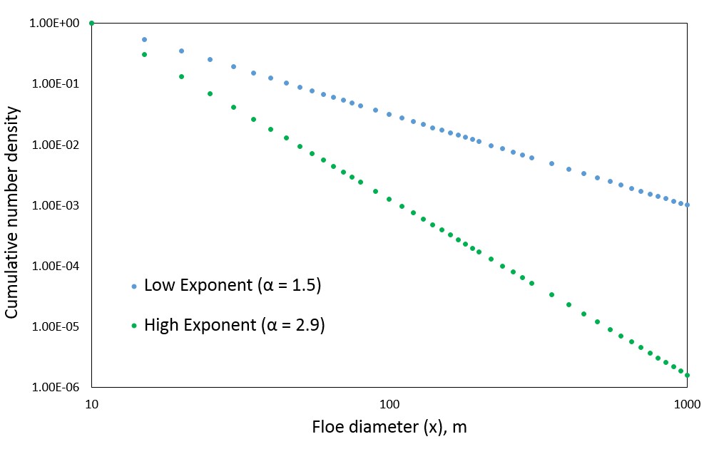
Figure 3: The cumulative number density for floe size can be represented by a power law. Note that both scales are log scales, and that C in the equation is a constant. The blue and green lines show the distribution for smaller and larger exponents respectively. Note the cumulative number density for a given floe diameter, x, is the fraction of floes size x and larger. [Credit: Adam Bateson]
The floe size distribution is most commonly fitted to a power law (Fig. 3). Power law systems have the property of self-similarity, a term attributed to a system which looks the same over different scales (e.g. the metre or kilometre scale). Power law distributions are relatively easily to investigate mathematically, and can easily be incorporated into a model without significant computational expense.
Do observations support the use of a power law?
Many individual experiments to assess the floe size distribution have shown a good fit to the power law. However, a large range of values for the power law exponent have been reported with observations ranging from 0.9 to 4. Other papers have proposed two power laws over different size ranges, with smaller exponents used for the smaller floe range. Herman et. al (2010) proposed that a distribution with a variable exponent would produce a better fit than a power law. There are further questions we need to consider as well. Over what scale are power laws a valid approximation? What determines the exponent of the power law and can it be assumed that this is constant? Is the power law only valid over a certain range of floe sizes and if so what determines this range?
These questions are not trivial, and the available observations are not sufficient to answer them. However, there is still value in testing different distributions and approaches within models. This can provide information about how sensitive the sea ice cover is to different distributions and which processes in particular are important to accurately model winter ice growth and summer ice loss in the marginal ice zone.
References/Further Reading
- Herman, Agnieszka. “Sea-ice floe-size distribution in the context of spontaneous scaling emergence in stochastic systems.” Physical Review E 81, no. 6 (2010): 066123.
- Horvat, Christopher, and Eli Tziperman. “A prognostic model of the sea-ice floe size and thickness distribution.” The Cryosphere 9, no. 6 (2015): 2119-2134.
- Williams, Timothy D., Luke G. Bennetts, Vernon A. Squire, Dany Dumont, and Laurent Bertino. “Wave–ice interactions in the marginal ice zone. Part 1: Theoretical foundations.” Ocean Modelling 71 (2013): 81-91.
- Williams, Timothy D., Luke G. Bennetts, Vernon A. Squire, Dany Dumont, and Laurent Bertino. “Wave–ice interactions in the marginal ice zone. Part 2: Numerical implementation and sensitivity studies along 1D transects of the ocean surface.” Ocean Modelling 71 (2013): 92-101.
Edited by Sophie Berger
 Adam Bateson is a PhD student at the University of Reading (United Kingdom), working with Danny Feltham. His project involves investigating the fragmentation and melting of the Arctic seasonal sea-ice cover, specifically improving the representation of relevant processes within sea-ice models. In particular he is looking at lateral melting and wave induced fragmentation of sea-ice as drivers of break up, as well as the role of the ocean mixed layer as either an amplifier or dampener to the impacts of particular processes. Contact: a.w.bateson@pgr.reading.ac.uk or @a_w_bateson on twitter.

![Lost in transl[ice]tion…](https://blogs.egu.eu/divisions/cr/files/2020/10/MainFigure-161x141.png)