The Polar Amplifier

Drip, drip, drop of the melting sea ice. Figure [Maria Scheel, imaggeo.egu.eu]

It’s no secret that the Arctic is warming faster than the rest of the planet, but why? Polar Amplification (often called Arctic Amplification) is the mechanism at play. In this week’s blog, we find out about its origins and why it happens.

Early Discoveries

In 1969, Russian scientist Mikhail Budyko and US scientist William Sellers discovered independently that the increase in greenhouse gases combined with the north-pole location of the sea-ice-covered Arctic Ocean and the tilt in the Earth’s axis led to an unusual arctic heating. The reason for this, they argued, was that as the concentration of CO2 and other greenhouse gases (methane, nitrous oxide, ozone) increased, so did the near surface air temperature. In the Arctic, the increase was approximately twice the equatorial increase (Lapenis, 2020; Budyko, 1972).

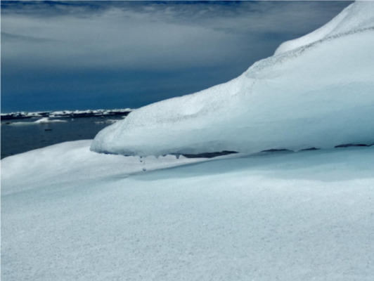
This means that in summer, as the arctic sea ice begins to melt and water replaces sea ice, the surface albedo increases from bright and reflective to dark and absorbing (see our other post on albedo here). The absorbed solar radiation then heats the atmosphere above the surface. This yields a positive feedback: As the warmer temperatures melt the ice, it retreats, expanding the area of enhanced surface temperature, which leads to a further retreat, and so on. This continues through the end of summer. Budyko and Sellers called this instability “Arctic amplification,” it is now called polar amplification.

Budyko further showed that if the concentration of greenhouse gases were to decrease, the process would run in reverse: Reduced radiative forcing would enhance the southward advance and growth of arctic ice. For extreme conditions, this could lead to “snowball earth.”

“Comparatively small changes in carbon dioxide concentration can considerably affect the mean temperature near the earth’s surface and result in the shift of polar ice cover over long distances.” (Budyko, 1972)

Using this instability, Budyko made a remarkable prediction in 1972 from a simple model based on a “business-as-usual” CO2 emissions scenario. He found that by 2050, sea ice would no longer cover the ocean year-round and that by 2070, the Earth’s mean global temperature would increase by about 2.25°C above its 1970 value (Budyko, 1972; Lapenis, 2020).

New discoveries

In recent years, many authors observed that another instability called the atmospheric lapse-rate feedback contributes to the amplification, where the lapse-rate is the decrease in temperature with height. For the lapse-rate, the differences in atmospheric moisture content, temperature, and circulation mean that the sign of the feedback changes from positive to negative between the tropics and poles. For the tropics as the surface warms, the feedback is negative and opposes the warming, for the polar regions, the feedback is positive. Although both the sea-ice albedo and lapse-rate feedbacks contribute to polar amplification, because the effects of the two terms are difficult to separate, considerable uncertainty exists about their relative magnitudes.

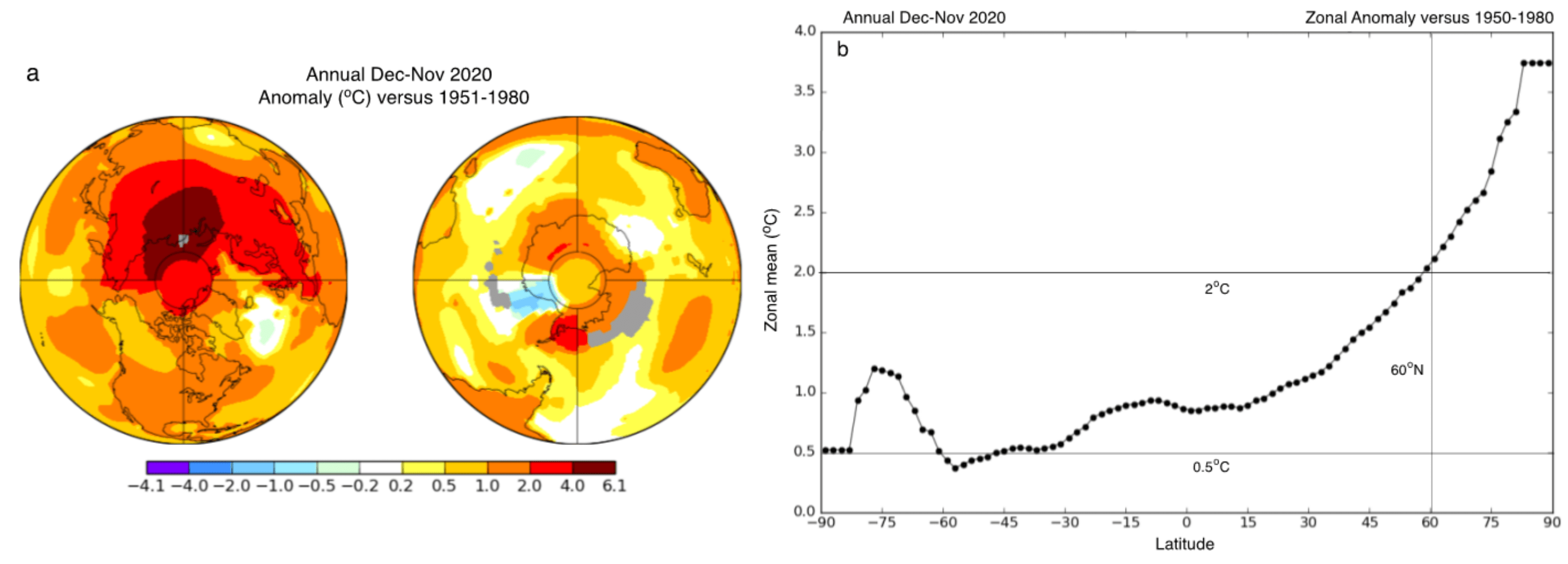
Figure 1. The 2020 annual average temperature anomaly relative to the period 1951-1980 derived from archived data. (a) Polar orthographic projections of the anomalies. (b) Zonal average of the anomaly (Figures derived from data and programs posted by the NASA Goddard Institute for Space Sciences (GISTEAM, 2021). [Courtesy NASA]

Arctic vs Antarctic

Figure 1 shows that for most of the Earth’s surface, the temperature increase in winter 2020 lies between 0.5 and 2oC warmer than the 1951-1980 average. But for the area north of 60oN, which contains 13% of the northern hemisphere area, the temperature increase approaches twice that, or between 2 and 4oC. The polar projection figure shows that for 2020, the temperature change is not evenly distributed, being strongest over Russia and Europe, and reaching a maximum of +6.1oC over Siberia and the adjacent Arctic Ocean. In the southern hemisphere, even though the continent and the sea ice remain too cold for the surface albedo to change, warming occurs over the Antarctic Peninsula and the Amundsen Gulf Embayment. These southern observations raise the question, if the lapse-rate instability occurs in both hemispheres, why aren’t the effects of polar amplification symmetric? In her 2006 post at the RealClimate website, Cecilia Bitz argues that while Antarctic amplification does occur, the upwelled deep water absorbs its heat.

For the Arctic, the strongest heating takes place not in summer (June-July-August), but in autumn (September-October-November). This is when the heat released by refreezing of the ice cover and by cooling of the summer heat absorbed in the water column is transferred to the atmosphere. At a slower rate, this warming continues throughout winter (December-January-February). As the sun rises in spring (March-April-May), solar radiation again becomes important and the heating increases, so that the maximum warming occurs in autumn and spring. This increases the length of the melt season compared to the non-amplified case (Stuecker et al., 2018).

Polar amplification affects both the arctic sea ice and its surrounding lands. The response of the sea-ice extent is the most obvious and dramatic. In 2020, the Arctic minimum sea ice extent was 65% of its 1980 value, and during the extreme 2012 sea-ice minima, it was 45% (NSIDC, 2021). The circumpolar lands are rich in permafrost and frozen organic material that contain about twice as much CO2 as the atmosphere (see our previous blog post on permafrost).

Further complications

For these lands, because the bare surface is dark and the snow is reflective, more solar radiation is absorbed and the land warms. As the permafrost thaws, CO2 and methane are released to the atmosphere. This release of greenhouse gases, although smaller than the anthropogenic release, still contribute to global warming and sea-level rise. Since these gases cannot be reinserted into the permafrost, their release provides another tipping point for the Earth system. The heating contributes to the Siberian, Canadian and Alaskan boreal forest fires, which directly emit CO2 and soot to the atmosphere, where the deposited soot may further contribute to the Greenland melt. Another change is that over the region, as the atmosphere continues to warm, rain replaces snowfall, yielding further regional complications (MacDougall et al., 2012; Quackenbush, 2021, McCrystall et al., 2021).

Lessons from the past

There are at least two examples of the importance of polar amplification in Earth’s climate history. These are the 125,000-year-old Last Interglacial (LIG) and the 3.1-million-year-old Mid-Pliocene Warm Period. Although these had similar CO2 concentrations to our present climate, the Earth’s orbital parameters were such that in both cases, the summer solar flux was brighter than present, and the sea level was higher. For the LIG, it was 5 – 10 m above present, and for the Pliocene, 11 – 21 m (CAPE, 2006; IPCC, 2021; Grant et al., 2019). During the LIG, the arctic summer temperature anomalies were 4–5oC above present and much greater than the average Northern Hemisphere anomaly. For these conditions, most of the Greenland ice cap melted, hippopotamuses lived in Britain, and boreal forests occupied parts of the area covered by the present Greenland ice cap. For the Pliocene, while its tropical temperatures were only slightly warmer than at present, arctic temperatures were much greater. For both periods, the tree line extended to the coast of the Arctic Ocean (CAPE, 2006; IPCC, 2021).

Polar amplification is a powerful regional instability that enhances the surface temperature over much of the northern hemisphere. It contributes to general climate woes such as the summer arctic fires, the release of CO2 from permafrost, and the melt of the arctic sea ice and the Greenland icecap. Its temperature elevation is more than twice the desired IPCC value of 1.5oC. The existence of this instability brings home the danger of further greenhouse gas emissions.