Lost in transl[ice]tion…

Further understanding of the Arctic sea-ice evolution is gained through satellite observations and climate models. Figure credit: C. Burgard & T. Finn.

Three years have passed since sea-ice scientists from both climate modeling and remote sensing backgrounds met for an international workshop in Hamburg. The goal was to discuss how to further improve our understanding of sea ice and reduce uncertainties in climate models and observations (see this previous post). One suggestion was to work on observation operators. Let’s see what has happened in the three years following this meeting…

The relationship between observed, simulated and real Arctic sea ice is ambiguous…

Three years is a long time, so let’s start with a short recap of the basics. In previous blog posts, we have shown you that the Arctic sea-ice cover is currently shrinking at a rapid pace due to climate change (see e.g. this and this previous post). To understand how the trajectory of the Arctic sea-ice cover will be in the next decades, climate scientists are using climate models to simulate future sea-ice evolution as a result of the CO₂ emissions predicted for the future. However, these climate models strongly disagree, resulting in a very large range of possible future sea-ice cover evolutions (the range is shown by the blue shading in Fig. 1).

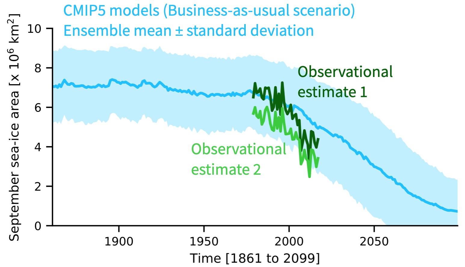
Fig. 1: Blue line = Mean evolution of the September sea-ice area as represented by global climate models from the CMIP5 generation, the model generation used for the 5th IPCC assessment report (the shading represents the standard deviation over all models) under the RCP8.5 scenario (often called business-as-usual scenario). Green lines = Evolution of the September sea-ice area from two different observational estimates of sea-ice concentration retrieved from the same satellite measurements (observational estimate 1 is retrieved with the Bootstrap algorithm, observational estimate 2 is retrieved with the NASA Team algorithm). Figure credit: C. Burgard.

To reduce this wide range of possible sea-ice evolutions, we usually try to identify the models that behave closest to reality. We do so by comparing the sea-ice concentration simulated by the climate models to observations. The most commonly used observations of sea-ice concentration (green lines in Fig. 1) are retrieved from brightness temperatures measured by passive microwave sensors on satellites from space. Brightness temperatures are a measure for the microwave radiation emitted by the Earth’s surface towards space.

And this is where the problem lies: there are different ways of “translating” the measured brightness temperatures into sea-ice concentration. This is because the translation depends not only on the sea-ice concentration itself but also on atmospheric, oceanic and sea-ice conditions, such as the surface temperature, the vertical structure and thickness of the sea ice, or the structure and thickness of the snow cover on top of the sea ice.

Different translators (called “retrieval algorithms”) can be applied to the brightness temperatures. Each of these translators uses slightly different assumptions to compensate for the missing information about the exact sea-ice, oceanic and atmospheric conditions. This means that each translation results in a slightly different sea-ice concentration (see Ivanova et al., 2014). Not knowing which of these sea-ice concentration estimates is closest to the real sea-ice concentration is a challenge when we want to evaluate the sea-ice concentration simulated by climate models (see Fig. 2, green arrows).

The observation operator, a potential solution?

One potential solution to overcome this challenge is the use of an observation operator. An observation operator is a tool that conducts reverse translations, i.e. it translates the climate state simulated by the climate model into a quantity that can directly be measured. In our case, it translates the simulated sea-ice cover and oceanic and atmospheric properties into a brightness temperature that could be measured by a theoretical satellite flying around the simulated Earth. The resulting simulated brightness temperature can then be compared directly with the measured brightness temperature (see Fig. 2, red arrows).

It is such an observation operator that I developed with colleagues. Let me tell you more about it…

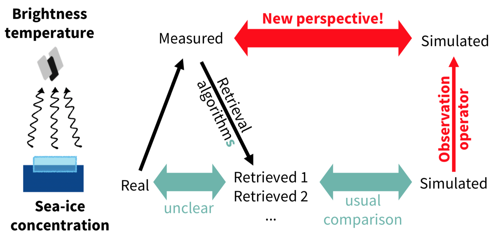
Fig. 2: Schematic showing the challenges linked to the comparison of simulated sea-ice concentration to observations of sea-ice concentration retrieved from satellite passive microwave measurements (green arrows) and how an observation operator would help circumventing these challenges (red arrows). Figure credit: C. Burgard.

Simulating realistic Arctic Ocean brightness temperatures from climate model output

But first things first: why would the translation from simulated quantity to observable quantity be less prone to uncertainties than the usual translation direction (from observable quantity to simulated quantity) you may ask? The answer is that a climate model provides a consistent climate state with the sea-ice concentration it simulates. The resulting brightness temperature is therefore also an accurate representation of all simulated sea-ice, oceanic and atmospheric properties influencing the brightness temperature. Remember: Having to assume some of these properties in retrieval algorithms leads to higher uncertainties when translating the brightness temperature into sea-ice concentration.

However, an observation operator has its own challenges. As mentioned earlier, the brightness temperature depends on the sea-ice and snow vertical structure. This is because the microwave radiation emitted by water (including sea water) and the microwave radiation emitted by pure ice are very distinct. Sea ice is a mixture of pure ice and brine, very saline water trapped inside the ice. Therefore, depending on the distribution of brine within the sea-ice column, the microwave radiation emitted at the surface varies. In snow, liquid water is present during melting periods. The effect of wet snow on the microwave radiation is so strong that it masks the radiation emitted by the sea-ice column below the snow. On top of that, when there is no water in the snow, the radiation is scattered by the snow crystals, which have a similar size as the wavelength used for retrieval algorithms.

The distribution of brine inside the sea ice, the detailed melt processes in the snow and the snow crystal size distribution and evolution are unfortunately not resolved in global climate models. While the crude representation of snow in climate models is a challenge that we cannot overcome at the moment, we can circumvent the snow “problem” by focussing our effort on a low frequency (6.9 GHz) only. At that frequency, the wavelength is high enough to ignore the influence of dry snow.

Concerning the vertical distribution (or profile) of brine in the sea-ice column, we conducted sensitivity experiments in an ideal one-dimensional setup. The brine profile mainly depends on the temperature and salinity profiles inside the sea-ice column. We show that we can infer simple vertical temperature and salinity profiles using the snow and sea-ice thickness and the surface temperature from the climate model output. With this simplified description of the sea-ice vertical structure, we can then calculate realistic sea-ice brightness temperatures. This approach works for freezing conditions, when the snow is dry (see Fig. 3, light blue box, “freezing conditions”). For the periods of higher temperatures when the snow or the sea-ice surfaces are melting, we find that information from below these melt surfaces cannot be used. In these cases, we propose using the following simple assumptions. For melting snow, we suggest that the brightness temperature equals the snow surface temperature (see Fig. 3, light blue box, “melting snow”). For melting ice conditions, we inferred a constant brightness temperature from satellite measurements over regions covered by 100% of sea ice (see Fig. 3, light blue box, “melting ice conditions”).

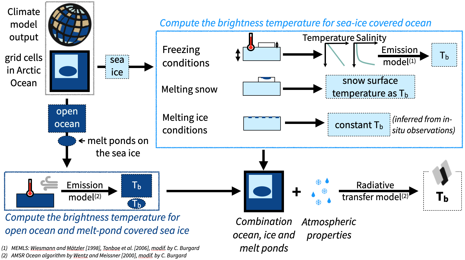
Fig. 3: Schematic showing the workflow of the Arctic Ocean Observation Operator for 6.9 GHz. For each Arctic Ocean grid cell, the operator calculates the brightness temperature (Tb) of the sea-ice-covered ocean surfaces (light blue box) and of the open-ocean and melt-pond surfaces (dark blue box) separately, then combines them, weighted with the sea-ice concentration, and adds the atmospheric contribution using a radiative transfer model. This results in the brightness temperature at the top of the atmosphere that would be measured by a satellite. Light blue boxes represent sea ice, white boxes represent snow, dark blue boxes represent water surfaces (open ocean and melt ponds on the sea ice). Figure credit: C. Burgard, inspired from Fig. 1 in Burgard et al., 2020b.

Once it was clear that we could simulate realistic brightness temperatures for sea-ice covered surfaces, we included the influence of open water surfaces in our operator, both open ocean (as the sea-ice concentration is not 100% everywhere) and melt ponds (areas of melt water that appear on the sea ice in summer). On top of that, we also added the influence of the atmosphere, which affects the radiation on its way between the surface and the satellite. We then extended the resulting tool from a one-dimensional framework to a multi-dimensional framework, so that it could easily be applied to climate model outputs, gave it a fancy name, “The Arctic Ocean Observation Operator for 6.9 GHz (ARC3O)“, and tadaaaa… we got our first set of simulated brightness temperatures that could be compared with measured brightness temperatures (see Fig. 4)!

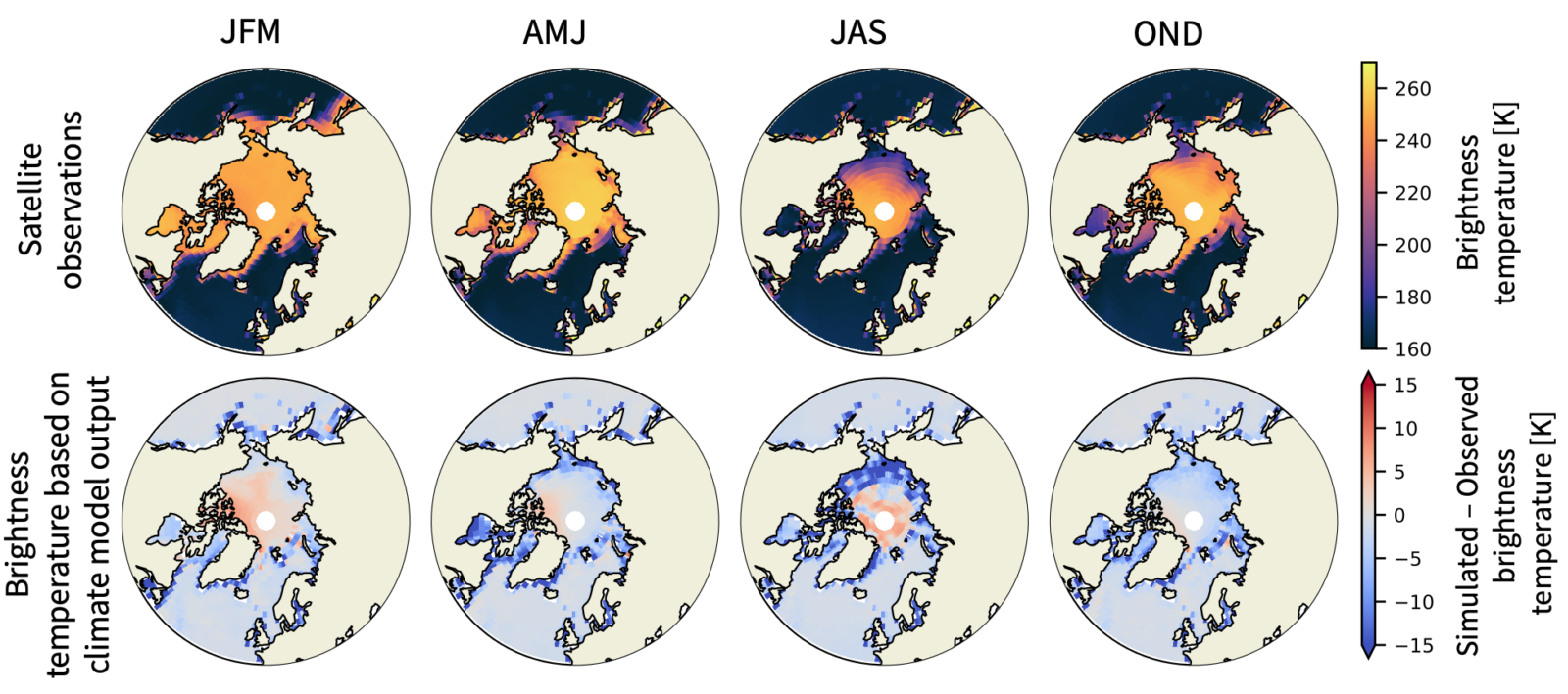
Fig. 4: Upper row: brightness temperatures at 6.9 GHz measured by AMSR-E from space. Lower row: difference between brightness temperatures simulated from climate model output and the measured brightness temperatures shown in the row above. The columns represent the seasons (JFM = January-February-March, AMJ = April-May-June, JAS = July-August-September, OND = October-November-December). Figure credit: C. Burgard.

And now?

As shown in Figures 2 and 4, we can now compare the simulated Arctic sea-ice characteristics directly to satellite measurements, circumventing the use of retrieval algorithms! While this brings us closer to reality, the comparison has its own challenges when it comes to interpretation. If the measurement and the simulation are different, this can be a result of an error in the simulated sea-ice concentration, but can also be an error in the sea-ice thickness, or the surface temperature, or other variables that we used in our translation from climate simulation to brightness temperature.

As an example: if you look at Figure 4, the overestimation in the simulated brightness temperatures in the central Arctic (red colors) in July-August-September could be a result of an overestimation of the sea-ice concentration or an underestimation of the fraction of melt ponds covering the ice. This is because melt ponds have the same (low) brightness temperature as open seawater. But which of the two it most likely is, we cannot know for now.

Still, this comparison provides an additional perspective when comparing climate simulations and observations, and also opens the possibility to investigate not only the simulated Arctic sea-ice concentration but other variables as well!

Further investigation into obtaining more detailed snow parametrizations might even enable us to include higher frequencies in the operator. As each frequency is differently sensitive to the sea-ice, oceanic and atmospheric parameters, combining several frequencies would help better pinpoint the source of differences between simulations and observations. Additionally, ARC3O could also be used in other contexts (e.g. data assimilation).

If you are interested to find out more, do not hesitate to contact me or play around with the Arctic Ocean Observation Operator, as it is now available as a python package 🙂