
Ice cores are important tools for investigating past climate as they are effectively a continuous record of snowfall, which preserves historical information about climate conditions and atmospheric gas composition. In this new “For Dummies” post, we discuss the history and importance of ice-core science, and look at the way we can use ice core chemistry to reconstruct past climate.
Ice sheets, archives of our past
When snow falls on the surface of an ice sheet it begins to compact the snow beneath it – eventually it will be compacted enough to be transformed into ice. Simultaneously, atmospheric air held between the snowflakes is slowly trapped in the ice – forming small air bubbles. In areas where mean annual temperatures at the ice surface remain below 0o C, such as Greenland and Antarctica, there is little surface melting, so this snow builds up to form thick ice sheets – up to 3000 metres in some part of East Antarctica! Low surface melt means that the snow that is compressed into ice each year forms a continuous record of the annual snowfall and atmospheric gas concentrations at the time of deposition, but how do we access this record..?
Snow that is compressed into ice each year forms a continuous record of the annual snowfall and atmospheric gas concentrations at the time of deposition
…We drill ice cores – of course!
An ice core is a cylinder of ice that is retrieved from the ice sheet by drilling vertically downwards. The core is drilled in sections from the surface, deep into the ice sheet (Fig. 1) using a rotating drill. Each section of the core is processed at the drill site and often cut further into shorter sections of ~55 cm for more practical transport and analysis in labs. A great deal of equipment is needed to achieve this and drilling is a slow and careful process often taking several field seasons to drill a deep core. An example of a drilling camp is shown in Fig. 2, housing scientists and engineers involved in drilling an ice core on the Fletcher Promontory, West Antarctica.
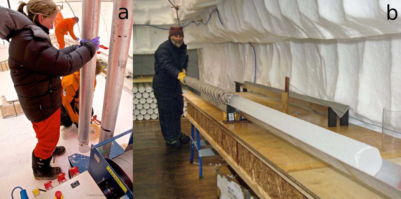
Figure 1: a) Ice core drill being lowered into the ice on Pine Island Glacier [Credit: Alex P. Taylor] b) Dr Rob Mulvaney processing the Berkner Island ice core, Weddell Sea, Antarctica [Credit: R. Mulvaney]
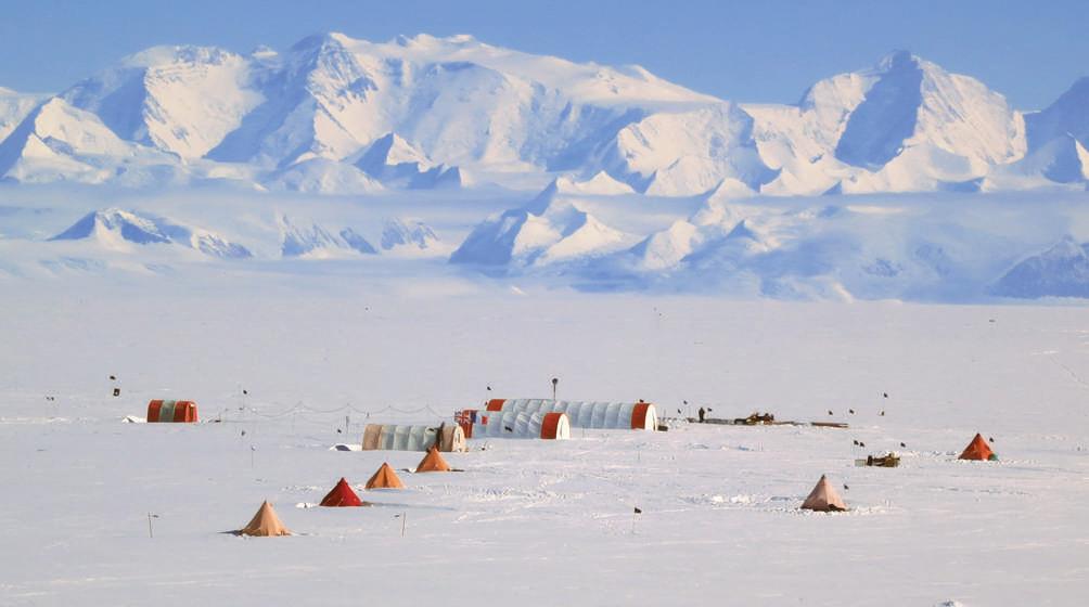
Figure 2: The layout of the Fletcher Promontory ice-drilling project, Weddell Sea, Antarctica. In the background the large Weatherhaven tent houses the drill rig, the central Weatherhaven tent is used for storage and equipment and a simple shower, the nearest Polarhaven tent is the mess tent, and the Polarhaven tent to the left houses the main generator. The pyramid tents in the foreground are the sleeping tents, and the two to the right are used for toilet facilities [Credit: Mulvaney et al., 2014]
Where to drill an ice core for the best record?
To get a good record of climate we want to find an area of ice that has many annual layers (good temporal resolution) that has not been disturbed by high ice flow velocities, usually these conditions can be found at an ice dome or divide. An ice sheet is a large plateau with a relatively stable rate of annual snowfall; the dome (or ice divide) is the point in the ice sheet where there is only vertical flow (compression) of ice (Fig. 3). Horizontal flow of ice is greater with the greater distance from the dome. Therefore, domes are the ideal site on the ice sheet or ice cap to drill for an ice core to ensure no interference with the snowfall history at the site. It is reasonable to assume that the ice-core record taken from a site with high annual snowfall will not extend the furthest back in time; similarly, a low annual snowfall and a large ice-sheet thickness will offer a record spanning much further back in time.
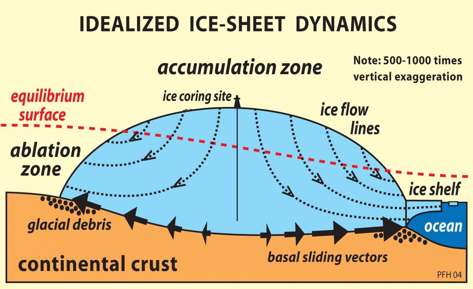
Figure 3: Ice flow within the ice sheet showing the zero flow at the ice divide – the ideal site for an ice core [Credit: Snowball Earth]
For Antarctica, the amount of snowfall across the ice sheet depends on the distance from the coast and sources of moisture; the highest mean annual snowfall is found at West Antarctic ice sheet sites whilst the lowest values are inland on the East Antarctic ice sheet, one of the driest deserts on Earth. In addition to the West and East Antarctic ice sheets, the Antarctic Peninsula is the third and final sector of the continent with high mean annual snowfall comparable to West Antarctica. In comparison to Antarctica, the Greenland ice sheet has a relatively high present-day mean annual snowfall, varying across the ice sheet between 10 and 30 cm per year. Therefore, if your aim is to find the oldest ice on Earth, East Antarctica is a good place to start looking, see our post on the quest to drill an ice core that contains ice which is over a million years old. Additionally, for the longest records it is paramount to find a drilling location with no (or at least very low) annual melting at the bedrock.
If your aim is to find the oldest ice on Earth, East Antarctica is a good place to start looking
What does an ice core actually record?
Once an ice core has been drilled and cut into sections, some of the sections are analysed and others are preserved. This is particularly important as some of the analysis is destructive (e.g. melting of the ice to extract water and gas). Therefore an archive of the ice core itself is needed. So, what information can we obtain from analysing the core and how is it done?
Annual layers, past snowfall and past temperatures!
Reconstructing the past surface temperature and snowfall is incredibly useful for understanding climate processes and changes through time in order to assess any present-day local and regional changes in climate. We can do this by:
- Measuring the thickness of the annual layers: This is done by counting layers in the core, either by visual identification of the peaks in deposition or use of a computer algorithm. The thickness of a specific year depends on how much snow fell at the site and on how much the snowfalls of the following years compacted this specific layer. We can estimate the strain caused by compaction which allows us to extract historical annual snowfall.
- Past air temperatures (Stable Water Isotope Record): An additional method to reconstruct past snowfall is from the ratios of the stable water isotopes from the water that forms snow and precipitation. The ratio of stable water isotopes has a linear relationship with surface temperature (see box below). Mathematical reconstructions of accumulation using the temperature reconstructions from stable water isotopes are employed in ice core profiles where the compaction of annual snowfall results in an annual layer thickness beyond standard laboratory resolution, such as Antarctic sites. Following the accumulation reconstruction, the rate of compaction of the annual snowfall to ice and subsequent ‘thinning’ of the deposited snowfall layer must be estimated by glaciological modelling.
- Trace-element analysis: For the upper depths of a deep ice core, or an ice core with an easily-resolvable annual layer thickness, the continuous analysis of an ice core for stable water isotopes offers a sub-annual view of the climate record.The deposition of a number of chemical elements increases during the summer season and decreases during the winter.When these elements are measured in the ice core they can be depicted as an almost-sinusoidal record, indicating the historical seasons. High-resolution ice-core profiles can be dated by counting these annual layers, and have been done so across Greenland and at the West Antarctic Ice Sheet (WAIS) Divide ice core site. Fig. 4 shows two annual signals over 24 months for four different chemicals that are deposited in ice cores (Sigl et al., 2016). The peak in seasonal deposition is shown twice for each chemical, at different times in history, but the seasonality of these species remains strong throughout time.
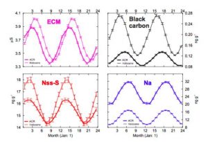
Figure 4: Seasonal deposition of four chemical species in the WAIS Divide ice core. Pink: electrical conductivity measurements; Black: Black Carbon; Red: non-sea salt Sulphur; Blue: Sodium. Each panel, shows the averaged annual record for 2 different periods: the Antarctic Cold Reversal (ACR, 13-14,000 years ago – bold line) and the Holocene, (10-11,000 years ago – thin line) the [Credit: Fig. 2, Sigl et al., 2016 ]
Reconstructing Past Temperatures
We commonly think of water as H2O - a molecule containing two hydrogen atoms and one oxygen atom. However, atoms (i.e. Hydrogen and Oxygen) come in several forms, known as isotopes - atoms with the same number of protons, but differing numbers of neutrons. Those isotopes that don't decay over time and are preserved in the ice core are know as stable water isotopes. It is possible to measure the amount of each different stable water isotope present in an ice core by melting the ice core and using a mass spectrometer to analyse the water produced.

The snow that eventually forms ice cores starts its life as ocean water which is evaporated and transported to the polar regions. Water isotopes with more neutrons are heavier and therefore require more energy to evaporate and transport. The amount of energy available to do this is related to temperature. Therefore heavier isotopes are found in ice cores in higher amounts at warmer periods in the planet's history! Find out more  here!
Atmospheric gas
Ice-core measurements of atmospheric gases correlate well with direct measurements taken from the atmosphere dating back to 1950. As a result of this, ice-core scientists can assume that the atmospheric gas concentrations measured in ice cores reflects the atmospheric conditions at the time the gas was entrapped in the ice core. Hence, ice cores tell us that carbon dioxide concentrations have been relatively stable for the last millennia until around 1800 AD but since then a rise of almost 40% has been measured in both ice cores and direct atmospheric measurements (Fig. 5).
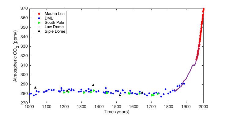
Figure 5: 1000 years of atmospheric CO2 concentrations from various Antarctic ice cores (DML, South Pole, Law Dome and Siple Dome) and the direct measurements in Mauna Loa Observatory [Credit: Ashleigh Massam, compiled from open access data sources]
Carbon dioxide concentrations have been relatively stable for the last millennia until around 1800 AD but since then a rise of almost 40% has been measured
In addition to comparison with present-day measurements, the trapped gases offer a record of direct atmospheric and greenhouse gas concentrations, including methane, carbon dioxide and nitrous oxide (Fig. 6) on a longer timescale – up to 800,000 years (Loulergue et al., 2008). Records show the connection between fluctuations in the atmosphere and long-term global climate variations (e.g. temperature) on a millennial timescale (Kawamura et al., 2007). The long-term trends show a pattern in the gas concentrations that compare well with glacial-interglacial climate. The phasing and timing of the eight glacial cycles covered by this record are dominated by the orbital cycle of the Earth on a 96,000-year periodicity, with a warm, interglacial period between each cold period. However, as we will see later in this blog post, this may not be the case when we look further back in time!
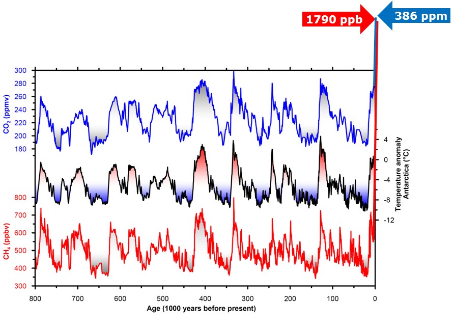
Figure 6: Variations of temperature (from present day mean temperature, black), atmospheric carbon dioxide (in part per million by volume — blue) and methane (in part per billion per volume red) over the past 800,000 years, from the EPICA Dome C ice core in Antarctica. Modern value (of 2009) of carbon dioxide and methane are indicated by arrows. [Credit : Centre for Ice and Climate , University of Copenhagen. Re-used with permission ]
Other climate proxies
Chemistry preserved in the ice also offers a proxy (=a means) to reconstruct other seasonally-deposited tracers:
- Information on past sea-ice extent can be obtained from chemicals found in ice cores which are also present in sea salt such as sodium, chlorine and methanesulphonic acid (MSA) (Sommer et al., 2000; Curran et al., 2003; Rothlisberger et al., 2003).
- The seasonal deposition of elements such as iron, magnesium and calcium, which are linked to dust from far-afield and the short-term climate variability such as atmospheric circulation (Fuhrer et al., 1999).
- Finally, volcanic layers in the ice core such as tephra and sulphate deposit provides a unique timestamp to a specific depth. These layers were deposited at the same time, all over the world and can be pinpointed to a specific volcanic eruption. Deposits of the same layer outside of a glaciated landscape, (e.g. within rock layers ) can often be dated using radiocarbon (Carbon-14) or another radiogenic dating methods. Additional age horizons can be interpreted by events assumed to occur in the world at the same time, such as rapid climate events. Age constraints are beneficial to interpreting deep ice-core records that are not analysed at a sub-annual resolution by offering pinpoint age horizons to an ice-core record.
Current knowledge from ice-core records
As we have seen, ice core are important because they put the current climate variations into the context of a long-term climate history. Additionally, polar ice cores can allow us to looks at variations between the northern and southern hemisphere. Ice cores also extend back much, much further in time than terrestrial weather stations or satellite records:
- 123,000 years for the northern hemisphere using the GISP2 ice core in Greenland (Grootes et al., 1993)
- 68,000 years at WAIS Divide in West Antarctica (Sigl et al., 2016)
- 800,000 years at Dome C in East Antarctica (EPICA, 2004).
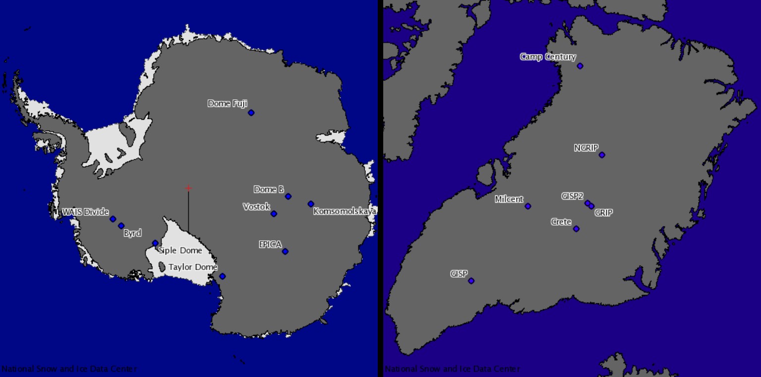
Figure 7: Deep ice core locations in Greenland and Antarctica [Credit and more details: NSIDC ]
The current past climate record tells us about glacial and inter-glacial periods (Fig. 6) but also allows us to look at finer detail – i.e. the variability within these periods, which were previously assumed stable. For example, ice cores have led to the discovery of Dansgaard-Oeschger events; which are are rapid climate fluctuation events, characterised by rapid warming followed by gradual cooling to return to glacial conditions, 25 of these events have happened during the last glacial period.
Records from the Northern and Southern hemisphere also allow us to link these small and large scale changes in climate in the two hemispheres. For example, ice cores analysed from both poles show a ‘call and response’ signal between Dansgaard-Oeschger events in the Northern Hemisphere and events in the Antarctic climate record. The southern hemisphere cooled during the warm phases of Dansgaard-Oeschger events in the northern hemisphere (Buizert et al., 2015), and vice versa during northern hemispheric cooling (see our previous blog post on the subject).
There are already over a dozen ice cores taken from Greenland and Antarctica (Fig. 7), offering a clear and detailed history of the climate during the Late Quaternary period (Fig. 6), going back up to 800,000 years (Quaternary = last 2.6 million years). As we mentioned earlier the timing of glacial and inter-galcial cycles in this 800,000 year old record is dominated by the orbital cycle of the Earth (96,000-year periodicity). However, marine records show that frequency of glacial-interglacial cycles was different before this time (Lisiecki and Raymo, 2005). It is in order to better understand these changes that the quest for the oldest was formed – beginning last month the mission aims to drill an ice core of ice older than 800,000 years to gain detailed information about the climate even further back in time.
Detailed records from high-resolution ice cores improves our understanding of the response of the planet to deglaciation events
The continuous and high-resolution of ice-core records, together with marine and terrestrial records, offers a global view of coupled processes from ice sheet calving events, changes to ocean circulation and heat transport and the subsequent cooling events across the Earth. Detailed records from high-resolution ice cores improves our understanding of the response of the planet to deglaciation events from the large ice sheets that once covered much of the northern hemisphere. Melting ice sheets pose a significant threat to the planet from rising sea levels and the freshwater input leading to inevitable changes in climate.
Edited by Emma Smith and Sophie Berger

Ashleigh Massam is a final-year PhD student based in the Ice Dynamics and Palaeoclimate group at the British Antarctic Survey and with the Department of Geography at Durham University. Her project is developing the age-depth profiles of three ice cores drilled at James Ross Island, Fletcher Promontory and Berkner Island, West Antarctica, by a combination of high-resolution trace-element analytical techniques and modelling ice-sheet processes.
Pingback: Climate change indicators/trends | Pearltrees
Pat Manning
A friend’s son in law, Bob Brett, is a helicopter pilot on the present Antarctic survey. He says Antarctic snowflakes differ from ours. Can you tell me in what way?
Thank you
Pat Manning
59 Staddiscombe Rs, Plymouth, UK
Pingback: Cryospheric Sciences | Image of the Week – The Sound of an Ice Age
Pingback: Cryospheric Sciences | A year at the South Pole – an interview with Tim Ager, Research Scientist
Pingback: Cryospheric Sciences | Image of the week – Learning from our past!
Pingback: GeoLog | GeoTalk: the climate communication between Earth’s polar regions
Pingback: Cryospheric Sciences | Image of the Week – Seven weeks in Antarctica [and how to study its surface mass balance]
Pingback: Cryospheric Sciences | Did you know… about the fluctuating past of north-east Greenland?
Pingback: Cryospheric Sciences | Did you know… that you can read the edge of Greenland’s ice as an open book?
Pingback: Cryospheric Sciences | Seafloor secrets: traces of the past Patagonian ice sheet