Did you know about the dark secrets of Arctic sea ice?

A map that shows the Thermal infrared tsurface temperature of the ice floe of the MOSAiC expedition in blue where its cold and red where it is warmer (leads).

Have you ever wondered what dark secrets the Arctic sea ice holds during the harsh winter months? Imagine total darkness in the central Arctic, making it almost impossible to gather scientific information. At this time of the year, usually only satellite observations are available. This changed in September 2019 when a team of scientists collected in situ and airborne data in the central Arctic as part of the year-long international MOSAiC expedition. In the following, I will show how we were able to study Arctic sea ice during winter and better understand a few physical processes of the Arctic climate system.

Helicopter-borne imaging during the polar night

My research is based on helicopter-borne thermal infrared imaging of Arctic sea ice. Now you might wonder what does thermal infrared imaging mean? A thermal infrared camera attached to a helicopter recorded thousands of images of the sea ice landscape underneath the helicopter. This happened during 35 helicopter flights during the winter 2019/2020 as part of the Multidisciplinary drifting Observatory for the Study of Arctic Climate, in short, the MOSAiC expedition. This expedition created a huge collection of interdisciplinary data sets during one full year in the Arctic, helping to better understand the Arctic climate system as it has never been done before. Most observations were focused on one large ice floe, called Central Observatory, to which the icebreaker RV Polarstern was attached while drifting through the Arctic Ocean. Getting back to thermal infrared cameras, unlike traditional visual cameras, they record the surface temperatures. You may ask yourself, why did they use this special camera? Because the Arctic winter during polar night means that no daylight available. Thus, all visual images would be black (check the NASA Worldview tool) and would not help to investigate the sea ice. To unlock a few of the sea ice’s dark secrets, we were able to study properties such as leads (linear cracks in the sea ice) and conditions that favor the formation of melt ponds (present in summer). You can see leads and melt ponds in Figure 1.

In this post, we will further explore these features and understand why they are important for understanding the behavior of Arctic sea ice. Join me as we delve into the world of thermal infrared imaging.

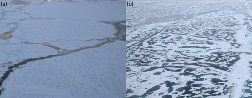
Two photos of cracks (leads) and melt ponds on sea ice.

Figure 1: Images from (a) leads and (b) melt ponds on sea ice taken from a helicopter in autumn 2020 during the MOSAiC expedition in the Central Arctic. [Credit: Linda Thielke]

Surface temperature maps

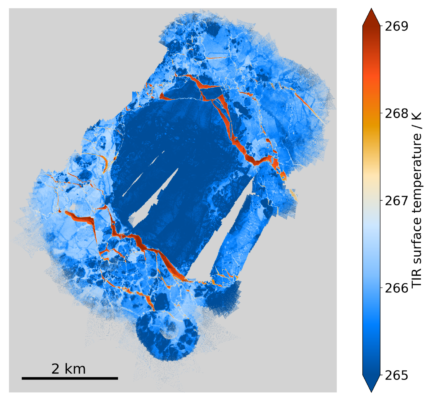
We generated a surface temperature map for each of the 35 helicopter flights, by stitching together all the thousands of surface temperature images at the correct location [Thielke et al., 2022]. Like this, we obtained a comprehensive view of the local and regional sea ice. The feature image displays the surface temperature map of 02 October 2019, showcasing the ice floe (dark blue) at the start of the MOSAiC expedition surrounded by thinner ice (lighter blue) and several leads (red). The helicopter-borne data has a limited spatial coverage ranging from local to regional scales (5 to 40 km), but a high horizontal resolution of 1 m, which allows us to see many details that may have gone unnoticed with pan-Arctic satellite data. These, in contrast, have a limited horizontal resolution of 1 km. One frequently used satellite product you might have heard of is the ice surface temperature from NASA’s Moderate Resolution Imaging Spectroradiometer (MODIS).

Small cracks in the ice – why are they relevant?

The detailed surface temperature maps allow us to study small-scale leads [Thielke et al., in review]. This is possible because leads, which expose the ocean to the atmosphere, are much warmer during winter than the surrounding thicker ice. Looking at the time series of the area fraction covered by leads during the MOSAiC winter, we found a varying area fraction of up to 4%, a considerable amount concerning the heat exchange from the warmer ocean to the colder atmosphere. Interestingly, we find more narrow (less than 10 meters) than wider leads (decreasing exponentially with increasing lead width), which was also found with other methods on different scales [Muchow, 2021]. This means that the helicopter-borne data include narrower leads than the satellite resolution (1 km). As both approaches are based on the same thermal infrared method, we can use the helicopter-borne data to evaluate satellite-based data for the MOSAiC helicopter flights. Our aim is to determine the role of narrow leads in the heat budget of Arctic sea ice.

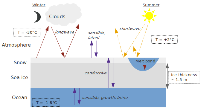
A scheme that shows a sun for summer and a cloud for winter and their thermal impacts in the snow, sea ice and ocean below.

Figure 2: Simplified scheme of the main processes involved in the heat budget across the Arctic sea ice. The arrows indicate the transport of heat via different fluxes that determine the heat budget in the ocean, the ice-snow pack, and the atmosphere. The indicated temperatures and ice thicknesses are examples of typical conditions. On the right side of the scheme, the additional summer fluxes (dashed) from shortwave radiation and melt are shown. [Credit: Linda Thielke]

Arctic heat budget of sea ice

As the Arctic warms up to four times faster than the rest of the world [Rantanen et al., 2022], a phenomenon called Arctic Amplification [Serreze, 2009] , which impacts the fate of ice in a changing climate. The sea ice heat budget, simply spoken, is the balance of heat fluxes determining the growth or melt of sea ice impacted by the ocean below and the atmosphere above. Ice thickness, snow depth, vertical temperature differences, presence of clouds, and many more aspects influence these fluxes, visualized in Figure 2. Temperatures at the snow/ice surface, as the interface with the atmosphere, play a crucial role in the heat exchange. Surface temperature maps are useful in capturing spatial variability since in situ measurements are typically point measurements. Later during summer, the shortwave radiation and the surface albedo become relevant and additionally influence the sea ice heat budget. The surface albedo refers to how much shortwave radiation is reflected; it is high for bright snow and low for dark surfaces such as melt ponds or open water.

How winter observations shed light on the summer heat budget

Based on the unique setup of the MOSAiC expedition, we can compare the same sea ice with helicopter-borne images from January (winter, surface temperature) and June (summer, visual images). That helped us to identify warm anomalies in the winter months that corresponded with the location of summer melt ponds [Thielke et al., 2023]. Why do we care? Melt ponds are a crucial component of the Arctic sea ice in the summer, decreasing the surface albedo and by that contributing to the ice-albedo feedback [Curry et al., 1995]. Hence, thermal infrared imaging helps us to understand the cycle of melt ponds better, which could help a better seasonal prediction of the behavior of melt ponds in the long run.

All in all, we learned about the potential of surface temperature maps from thermal infrared imaging, particularly about small leads and melt ponds as they are crucial for the Arctic heat budget. For the future, this knowledge can be used to improve climate model simulations.