Mapping sea ice from space

Figure 1. The thinning and retreating of sea ice have led to increased human activity in Arctic waters. Hence, marine traffic and activities such as fishing, shipping, oil and mineral exploitation are expected to increase in the future. To handle navigation in ice-covered waters, vessel crews need appropriate planning support. [Credit: Alex Perz/Unsplash]

Reduced and thinner sea ice makes Arctic waters increasingly appealing for shipping, fishing, tourism, and mineral exploration. However, with increased accessibility and more dynamic ice conditions comes a greater risk for ship crews to encounter sea ice and icebergs outside of their usual seasonal limits. To help them navigate, timely and reliable sea ice information is key. Have you wondered how sea ice information can be provided for vast and remote areas such as the Arctic Ocean? Read on when you are curious to learn about mapping sea ice from space!

Introduction

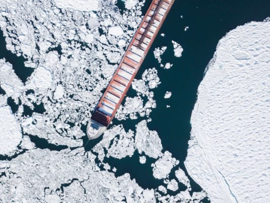
We are on the bridge of KV Svalbard, somewhere North of Svalbard, conducting a scientific cruise led by the Nansen Environmental and Remote Sensing Center (NERSC). The cruise was part of the Useful Arctic Knowledge (UAK), Integrated Arctic Observation System (INTAROS) and Digital Arctic Shipping projects and had participation of 12 PhD and master´s students from seven countries.

It is mid-June, and yesterday’s clear and sunny weather changed into thick foggy greyness. Visibility is low, the sea is flat and, looking at where the horizon used to be, one can barely tell where the ocean ends and the sky begins.

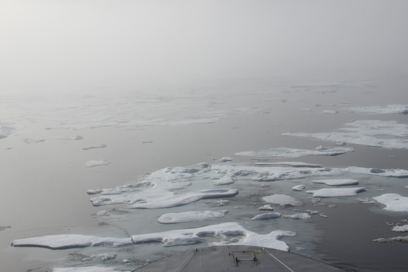
Figure 2. A view of KV Svalbard´s path ahead on a foggy day in the Arctic Ocean north of Svalbard. [Credit: Ole Jakob Hegelund/IceWatch]

Something brighter than the ocean surface seems to appear in the distance. Is it a ship, an iceberg, or sea ice? Binoculars don’t help much, but the navigation charts tell us it cannot be an island. The vessel slows down, and our eyes are moving between the vast greyness ahead and the bright and flickering screens in front of us at the bridge. What will we find ahead?

The perks of sea ice

Sea ice is a fascinating and dynamic part of the polar environment and the Earth’s climate system. It plays an important role in the global climate system through its ability to reflect sunlight and has a natural cooling function.

The sea ice in the Arctic changes with the seasons. New ice forms during cold periods, grows thicker over the winter months, is squeezed into thick ice flows and ridges, or it breaks apart and melts in the Arctic summer. Wind, ocean currents, and waves constantly move the ice too, which adds to the dangers of travelling through it.

Small and large icebergs frequently break off from glaciers around Greenland and Svalbard and float through the icy Arctic waters. Both sea ice and icebergs travel over large distances with ocean currents, winds and waves before they eventually melt, or are pushed and squeezed into more dense and thick ice or pressure ridges.

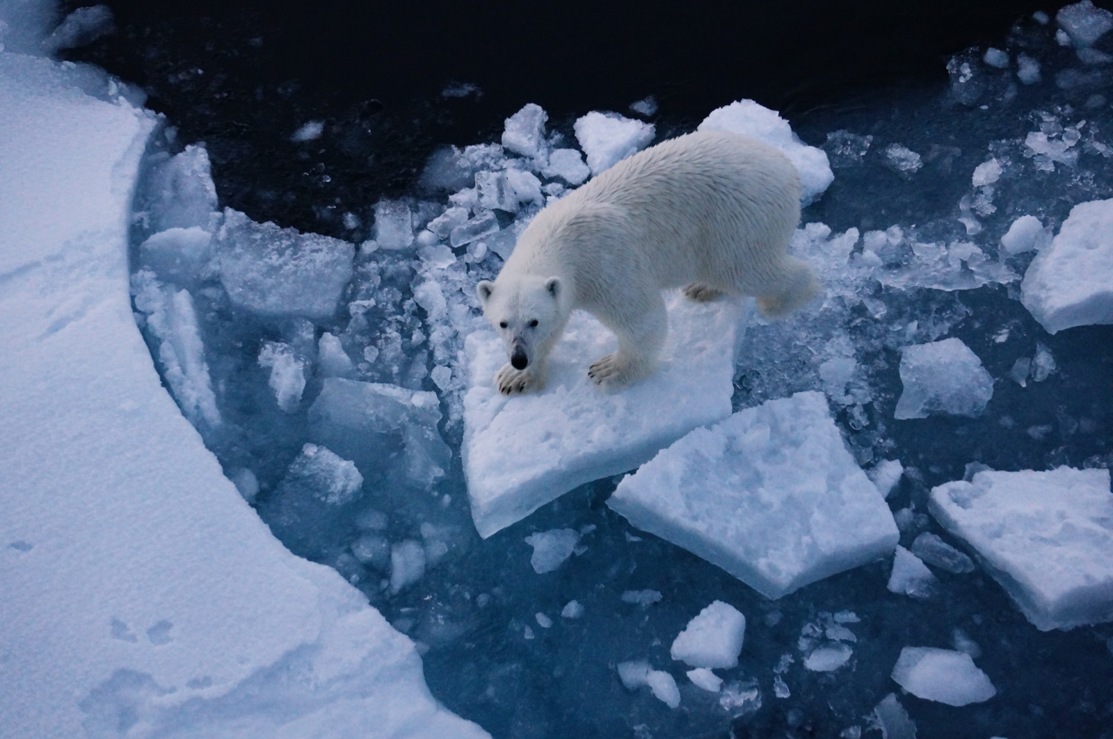
Figure 3. Sea ice is also an important part of polar ecosystems: the ever-changing sea ice edge allows light to enter the water beneath so that tiny algae can grow. These algae provide food for marine animals, fish, birds and mammals such as seals and polar bears. [Credit: Anca Cristea/Norwegian Polar Institute]

Increased human activity in icy waters

Less and thinner sea ice makes Arctic waters increasingly appealing for human activity such as shipping, fishing, tourism, and mineral exploration. Ocean areas that were previously covered by thick and dense sea ice now have a thinner ice cover and are becoming more and more accessible. Some of these places are still uncharted, with the seabed conditions unknown, and others are open water or covered by loose sea ice. However, sea ice can drift fast and can damage vessels and offshore structures.

Reduced sea ice enables human activity in the summer season, while we know little about the winter sea ice conditions in the central Arctic. The MOSAiC expedition to the central Arctic Ocean (2019-2020) followed Nansen`s Fram expedition. On its 3.400 km drift through the Arctic, it collected new data and insights about how sea ice forms and interacts with the climate and ecosystem. This helps mapping sea ice particularly in the winter months where data are scarce.

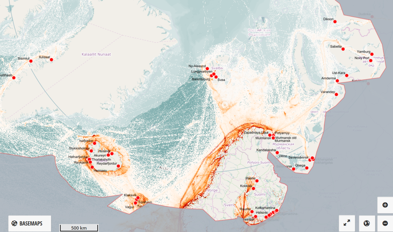
Figure 4. Arctic ship traffic map showing ship tracks in the Barents Sea and adjacent shelf seas – which are the focus area of CIRFA – from July 2016 to July 2017. The orange lines are ship tracks, the red dots are harbours. [Credit: PAME – Arctic Ship Traffic Data]

Increased safety for polar marine activities

Far from civilization with few icebreakers around to help, without being at risk of being enclosed by thick sea ice or unexpectedly meeting an iceberg – how can vessels safely navigate? What types of sea ice are out there in the Arctic Ocean? Where are they located, where are they drifting to, and how fast are they moving? How can we map sea ice in all its forms to help ships decide the best and safest course? How we do this efficiently for large and remote areas? There are many questions to address!

The traditional way of mapping sea ice relies on visual analysis and interpretation of radar satellite images by sea ice analysts. The results of this analysis are then provided to the ship captains in the form of sea ice type or sea ice concentration maps. However, manual production of these maps is a time consuming and arduous task.

Researchers at UiT and the partners in CIRFA are developing new ways to identify sea ice conditions. We use data from radar instruments carried by satellites such as the European SENTINEL-1 and Canadian RADARSAT-2. The satellites cross over the Arctic several times a day and scan the ocean surface in beams that can be up to a few hundred kilometres wide. In contrast to optical sensors, the radar can see the ocean surface through clouds and in darkness.

New ways to make sea ice maps

Instead of visually interpreting each satellite image, researchers at CIRFA and MET have developed an algorithm that automatically interprets many satellite images at a time. The algorithm built by CIRFA researchers Johannes Lohse, Wenkai Guo and Anthony Doulgeris can recognize different types of sea ice. Its ability to do this is rooted in the physical properties of the backscatter; the strength of the radar signal that is reflected from the Earth surface and recorded by the satellite.

To understand how backscatter works, imagine how the light of a flashlight reflects differently depending on what you shine the light on. Like smooth surfaces appearing bright and corners or edges making shadows, the reflected radar signal depends on whether the water or ice is rough and deformed, or if it’s smooth, almost like a mirror. The change in backscatter, if properly analysed, tells us about different sea ice types and open water areas.

To automatically process the satellite data and make ice type maps, the algorithm was optimized over months. During this optimisation, the researchers trained the algorithm by showing it a lot of data corresponding to different sea ice types recovered from manually analysed satellite images. This step is essential to gain confidence that the algorithm can distinguish and map smooth or deformed sea ice, wet surfaces, sea ice ridges, and open water areas.

The algorithm can make a map based on satellite imagery for a specific location, for example in the northern Atlantic Ocean, in as little as 15 minutes. For larger areas, or areas that are not as frequently overflown by satellites, it will take more time to acquire data and make maps.

Testing the algorithm in real conditions

PhD candidates Anna Telegina, Jozef Rusin and Laust Færch, and the Norwegian Meteorological Institute (MET) engineer Alistair Everett joined the UAK research cruise on KV Svalbard in June 2021 when CIRFA’s automatic sea ice classification was tested. Before and during the cruise, the algorithm was set up at MET, where the latest satellite images were analysed and the ice type maps were produced before they were sent to the ship. The team on the ship compared the sea ice maps generated by the algorithm with reality around the vessel to check and confirm the information from the algorithm.

In addition, Tom Rune Lauknes from the Norwegian Research Center used drones to map sea ice with ultra-high resolution optical images. This is important to correctly characterize the ice, to learn how well the algorithm works, and to know how to improve it.

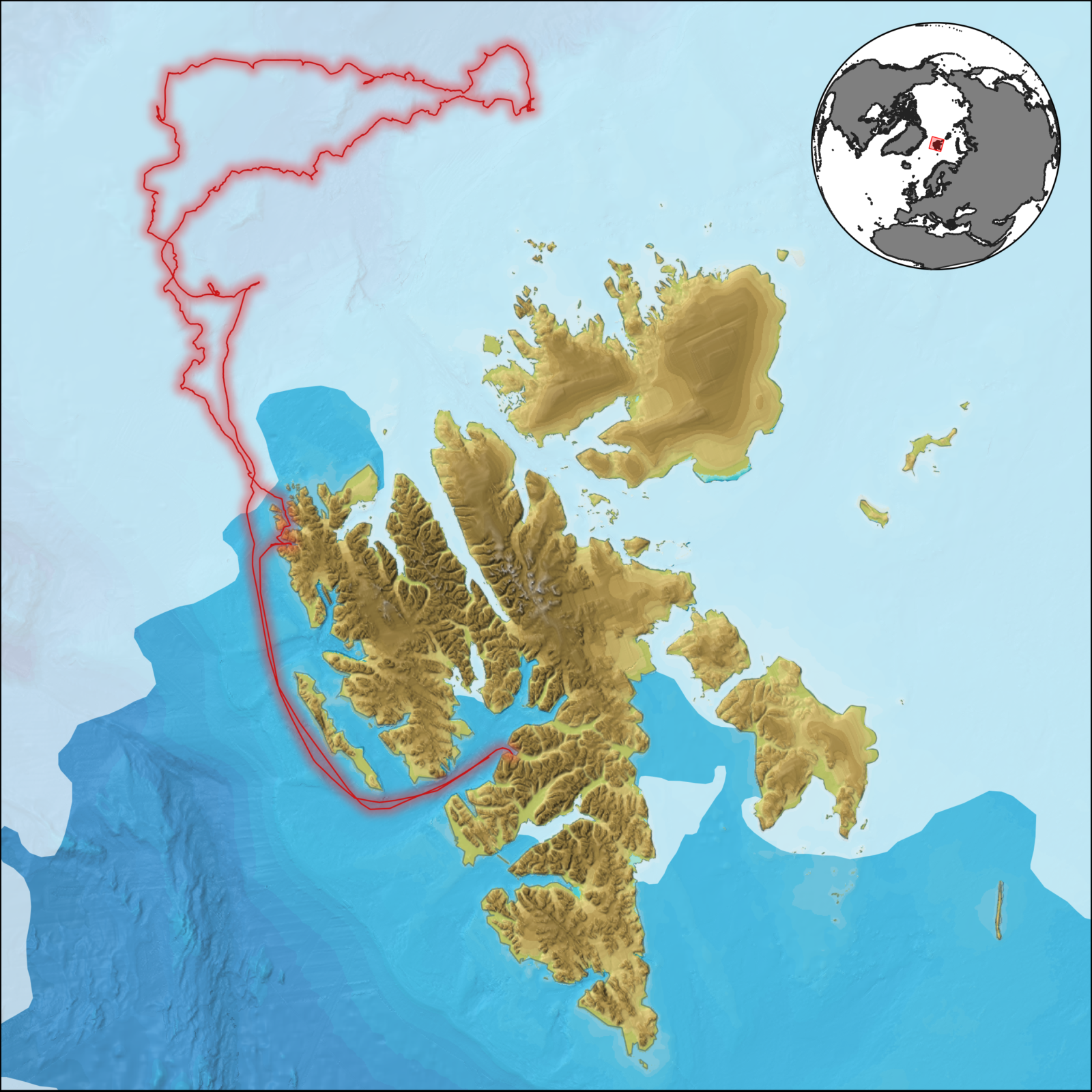
Figure 5. The algorithm was tested during a research cruise North of the Svalbard Archipelago in June 2021. The light blue area shows the ocean that is covered with sea ice at this time of the year while the dark blue area is open water. The ship track is outlined in red. The map is based on bathymetry data from IBCAO v4. [Credit: Alistair Everett/MET]

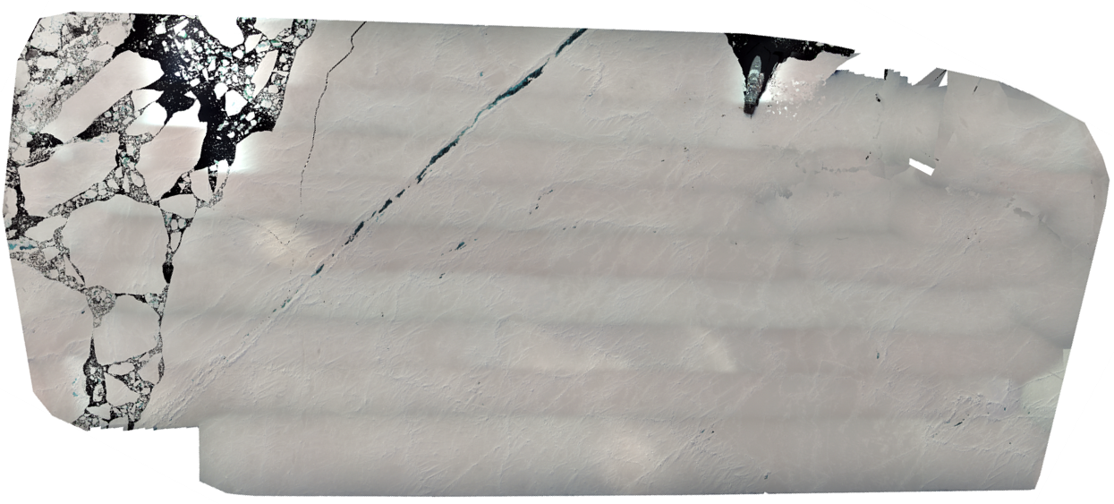
Figure 6. Drone orthomosaic of the fieldwork area. KV Svalbard was attached to a large ice floe with ridges of drifted snow or pressure ridges, and a large crack and open sea ice on the left side. [Credit: Tom Rune Lauknes/NORCE]

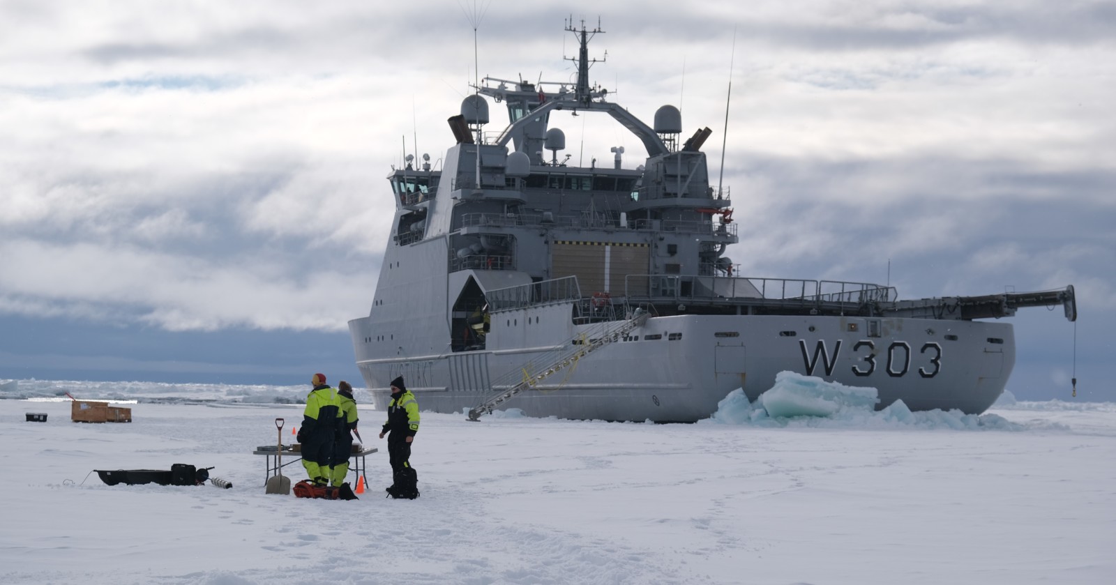
Figure 7. In addition to making ice observations from satellites, drones and the bridge, the team investigated ice properties such as density and salinity by drilling ice cores and studied the snow lying on top of the ice. The team is shown with KV Svalbard in the background. [Credit: Jozef Rusin/MET]

The researchers were pleased with the positive results: the algorithm interprets the satellite data well and detects different ice types that the researchers on-board confirmed. Based on the simultaneous feedback, the algorithm could even be improved during the ongoing cruise.

However, a lot more research and fieldwork are needed for automatically made ice maps to become a reliable source of information. Looking further ahead, automatically generated sea ice information on a regional and pan-Arctic scale will ease decision-making in navigation, search-and-rescue and other maritime activities in remote, ice-covered waters.

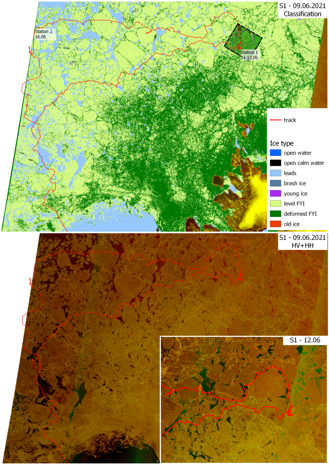
Figure 8. Top: Example of the sea ice classification in satellite images North of Svalbard. The different colours represent different ice types and open water. Bottom: In the Sentinel-1 satellite false-color image, sea ice appears as green/brown areas while open water as dark areas. The red line outlines the track of KV Svalbard. [Credit: data used to produce this figure come from Sentinel (Copernicus) and Radarsat-2 (NSC/KSAT under the Norwegian-Canadian Radarsat agreement 2021) data. The maps are made by Anna Telegina and Johannes Lohse/CIRFA]

Challenges for early polar travel

Leaders of historic expeditions to the Arctic and Antarctic soon became aware of the dangers of sea ice and icebergs.

For example, the Norwegian-Belgian Belgica expedition to Antarctica (1897–1899) was trapped in the sea ice for 377 days and drifted with it for over 3000 km until the up to 4 m thick ice around the vessel loosened up and released the ship. The Endurance expedition to Antarctica (1914–1917) was less fortunate. Despite having a special hull designed to withstand polar conditions, pressure from the surrounding sea ice eventually crushed the ship. The expedition photographer Frank Hurley captured the sinking vessel in photos that were later turned into a video.

Remains of the American vessel Jeannette, which had sunk off the north coast of Siberia in 1881 after being trapped and crushed by sea ice, were discovered a few years later off the south-west coast of Greenland. Finding the ships’ remains in Greenland inspired the idea of an ocean current flowing from east to west across the polar sea (today known as transpolar drift. This gave the Norwegian explorer Fridtjof Nansen the idea that a properly constructed ship could enter the Arctic Ocean in the east, survive the pressure during the drift, and emerge in the northern Atlantic Ocean, perhaps having even traversed the North Pole. This theory was the basis of Nansen’s Fram expedition of 1893–1896.

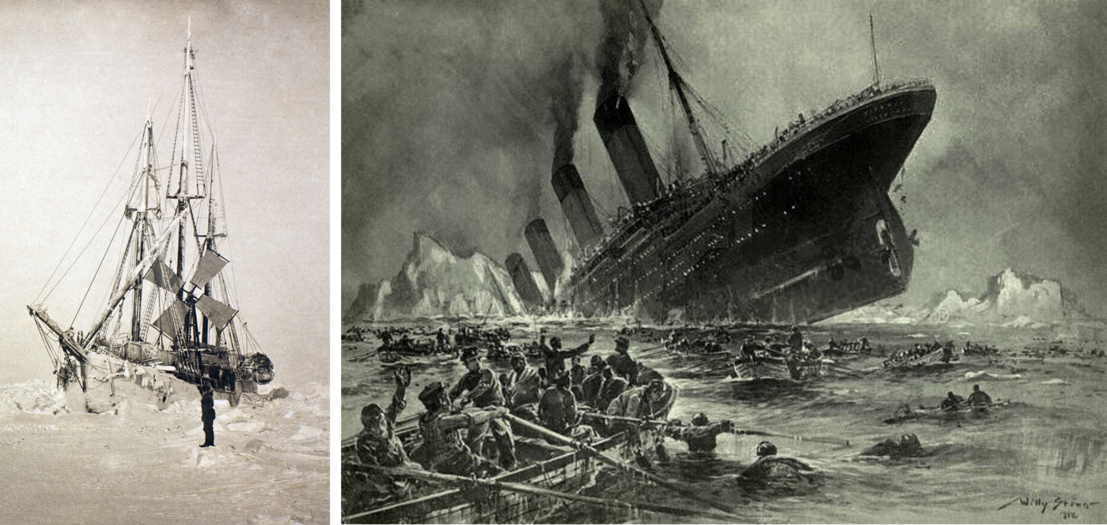
Figure 9. Sea ice and floating icebergs have early been recognized as a hazard for historic expeditions and passenger travel. Left: The Norwegian expedition ship Fram in the Arctic sea ice in March 1894. [Credit: Scanned from Nansen: Farthest North, Constable, London 1897]. Right: A collision with an iceberg made the Titanic sink on its maiden voyage. [Credit: Titanic Sinking, engraving by Willy Stöwer]

Floating icebergs have also proven problematic for travel. The maiden voyage of the Titanic in 1912 is anchored to the public historic memory as a tragedy caused by a collision with a drifting iceberg. The iceberg was likely part of a Greenlandic glacier. It was seen too late by the Titanic’s crew; too late to slow down and turn the heavy ship; too late to safely navigate around the icy giant whose real dimensions are mostly hidden under the water surface.

If ice maps would have been available in the 19th and 20th century, things may have ended differently.

About us

The Norwegian Coast Guard is acknowledged for providing 14 days of shiptime with the icebreaker KV Svalbard, which made it possible to conduct the cruise in the sea ice areas north of Svalbard.

The Nansen Environment and Remote Sensing Center (NERSC) organised the cruise and the measurement programme. The goal of the Useful Arctic Knowledge: partnership for research and education (UAK) project led by NERSC is to develop long-term collaboration between Norway, Canada and USA to improve multidisciplinarity in Arctic research and education. UAK is funded by the Research Council of Norway (grant no. 274891).

CIRFA (Centre for Integrated Remote Sensing and Forecasting for Arctic Operations,) conducts innovative research and education in satellite remote sensing and numerical modelling to support high-latitude marine activities and environmental monitoring. CIRFA is funded by the Research Council of Norway (grant no. 237906).

The Norwegian Meteorological Institute (MET Norway) is Norway’s national meteorological institute and runs the Norwegian Ice Service.

The H2020 project INTAROS – Integrated Arctic Observation System develops improved observing systems in the Arctic (http://intaros.eu, http://intaros.nersc.no). INTAROS is funded by EU under contract no 727890.

The project Digital Arctic Shipping develops new sea ice data products and visualisation services for Arctic shipping. The project is funded by RCN contract no. 309708.

The Norwegian Research Center (NORCE) was responsible for the drone programme.

IceWatch is an observation and data network program to help monitor Arctic sea ice. It is an open-source forum to facilitate the collection and sharing of near-real time ship tracks and sea ice conditions throughout the Arctic Ocean.