From Fault Architecture to Grain-Scale Deformation: Integrating Field, Microstructural, and Experimental Approaches

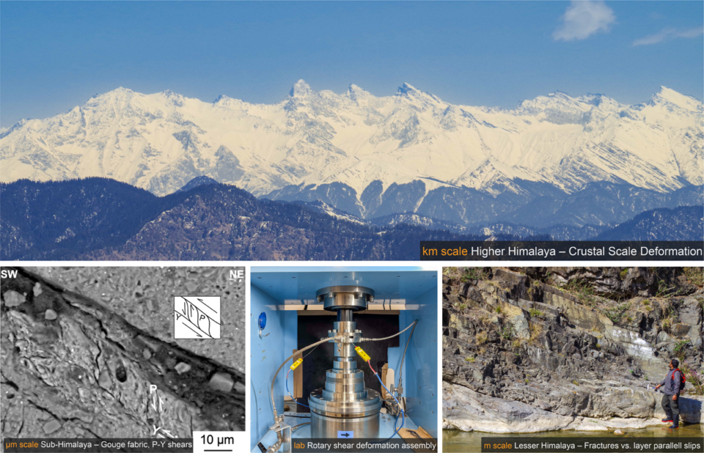
Fault zones are far more complex than the lines we draw on geological maps. Their internal structures, mineralogical compositions, and deformation histories offer important clues to deformation mechanisms and even how earthquakes might occur. But how can we connect what we observe in the field with the microscopic processes and mechanical behaviour of faults at depth? In this blog, we explore how combining field observations, microstructural analyses, geochemical methods, and laboratory experiments help unravel the complexities of fault deformation.

What does a fault zone look like, and how does it grow?

I started where most structural geologists start– in the field. During my master’s research, I focused on paleostress estimation from mapping the outcrop-scale fracture and faults occurring within the Himalayan Frontal Thrust region, a classical structural approach. Doctoral research, deepened this field-based approach across the major thrust systems of northwestern Himalaya – the Main Frontal Thrust, the Nahan Thrust, and the Main Boundary Thrust (Figure 1). Systematic outcrop mapping, combined with microstructural and mineralogical analysis using SEM-EDS, XRD, and EBSD, revealed the heterogenous structure of fault zones even at outcrop level (Sarkar et al., 2022). Adjacent rock layers with different mineralogies develop fundamentally different fault fabrics – foliated gouges in phyllosilicate-rich layers, cataclastic gouges in quartz-dominated sandstone layers. Slip localization at the boundary between these distinct litho-domains, recorded in the rock as ultrafine bands, amorphous materials, vapor escape structures, and clay clast aggregates (Sarkar et al., 2022).

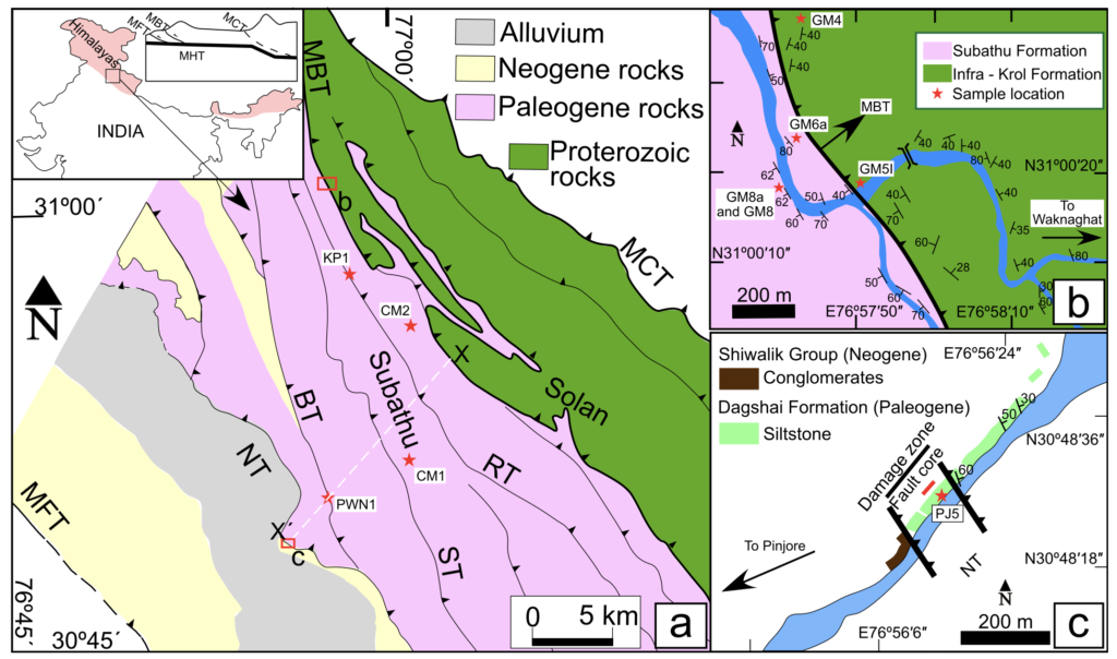
Figure 1. (a) Regional geological map of the northwestern Himalaya, modified from Saha et al. (2016). The inset illustrates the location of the study area and a simplified schematic cross-section of the Himalaya after Bose et al. (2009). Abbreviations: MHT: Main Himalayan Thrust; MCT: Main Central Thrust; MBT: Main Boundary Thrust; RT: Ranon Thrust; ST: Surajpur Thrust; BT: Bilaspur Thrust; NT: Nahan Thrust; and MFT: Main Frontal Thrust. Sample locations are marked by red stars. The red rectangles indicate the areas enlarged in panels (b) and (c). (b) Geological map of the MBT at Gambarpul showing sample locations and bedding orientations. (c) Geological map of the NT displaying lithological variations, sample locations, and bedding orientation data.

At what temperature and depth did these faults slip?

Characterizing fault architecture raises an immediate question about the physical conditions under which deformation occurred. In the shallow Himalayan thrust belt, rocks are unmetamorphosed to low-grade, so conventional geothermometers based on metamorphic mineral assemblages are often inapplicable. Combining carbonate clumped isotope thermometry with calcite e-twin morphology (Sarkar et. al. 2021) provided a way forward. Applied to syn-tectonic calcite veins across the Himalayan frontal wedge, this approach constrained formation temperatures and depths for two major thrust systems, establishing an inverted thermal gradient consistent with thrust loading and rapid exhumation. This was one of my first applications of clumped-isotope thermometry directly to shallow crustal fault rocks in an active orogenic setting (Sarkar et al. 2022).

Where exactly is the fault, and how do we find it?

Identifying the precise location of a major thrust is not always straightforward. In one study area along the Main Boundary Thrust, the contact was not expressed by characteristic fault rocks at the outcrop scale. Detrital zircon U-Pb geochronology of sandstone and siltstone samples from both sides of the suspected contact resolved this problem (Sarkar et al., 2023). A sharp change in maximum depositional age – from Neoproterozoic in the hanging wall to Cenozoic in the footwall – pinpointed the thrust contact to less than one meter and provided new constraints on the stratigraphic identity of the hanging wall rocks.

What controls whether a fault creeps or ruptures seismically?

Field observations and microstructural data establish what happened in a fault zone. Friction experiments address why. Using a rotary shear apparatus (Figure 3), I conducted room-temperature friction experiments on natural sandstone and fault gouge samples from the Main Frontal Thrust, spanning slow creep velocities of 10–200 μm/s through to seismic slip rates of approximately 1.5 m/s (Sarkar and Hirose, EGU2023). Samples with higher phyllosilicate content showed velocity-strengthening behaviour, while those with lower phyllosilicate content showed initial velocity-weakening. This directly links the mineralogical heterogeneity of the protolith to the possible partitioning between seismic and aseismic slip within the same fault zone. XRD analysis further showed that phyllosilicate content, increases during slip even at room temperature experiments, suggesting that fault zones may progressively evolve toward more stable sliding behaviour as deformation accumulates.

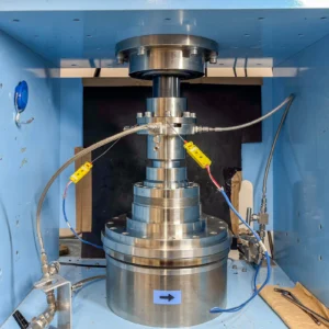
Figure 3. The rotary shear apparatus housed at JAMSTEC Kochi Core Centre in Japan.

The broader picture

Across the research stages, the central question has remained constant: how do faults deform across the seismogenic zone, and what controls the transition between stable creep and seismic rupture? Field mapping, microstructural analysis, isotope thermometry, geochronology, and friction experiments each illuminate a different aspect of this problem. Together, they build toward a more complete understanding of fault rheology in active collisional settings.