Nuno Simões
University of Algarve, Portugal
E-mail: nuno_simoes58@hotmail.com

Nuno Simões (before combing). Meet Nuno at EGU2014-SSS2.7.
We can easily see that soil color varies from one site to another, with depth, with topographic position and composition. Even color may be light brown in one side of the road and dark brown in the other. Whether for scientific purposes, or just curious, you study the colorimetric interesting variations.
Why does soil color change?
The soil color varies due to the characteristics of substances that form it. These variations can be caused by several factors, as, for example, soil humidity (the wetter the soil is, the darker it gets), soluble salts, sand and carbonates (light colors), iron oxides (red colors), organic matter (dark colors), etc.
How can soil color be measured?
Soil color is usually described using the Munsell color scale, which is a very good tool for soil taxonomy, for example. But there are other interesting methods that can be used depending in our purposes. The method I am presenting here uses the ColortronTM spectrophotometer, a device that measures the color at the surface of solids and transfers it to the ColorshopTM program. This spectrophotometer can use various color scales such as CIE Lab, CIE RGB, CIE XYZ, among other scales.
A study case
This example is a study conducted in Boca do Rio (Algarve, southwestern Portugal), which consisted of the identification of sedimentary deposits of the 1755 tsunami in the area. We used the CIE Lab color model which, according Nederbragt and Thurow (2004), is the most suitable for paleoenvironmental studies. CIE Lab aims to mimic the way the human eye understands the color and is divided into three parameters, L*, a* and b*. This color space is organized in a three-dimensional model, where L* is the vertical axis and is defined by lightness (Figure 1). The maximum brightness is L* = 100, which represents a perfect diffuser (reflecting white) and the minimum is 0, which represents black. Value of L* is conditioned by organic matter and carbonate contents (Helmke et al., 2002), as well as water content. In contrast, a* and b* represent the chromaticity and do not show numerical limits. The value of a* is positive when it tends towards red, and negative when it tends towards green. Similarly, b* is positive when it tends to yellow and negative when it tends to blue.

Figure 1. CIE Lab scale.
How to?
Usually, three replicated color measurements are carried out with the Colortron and average values are used as representative.

Figure 2. Sediment sampling.

Figure 3. Sediment samples prepared to start measuring (left) and Colotron device (right).
After obtaining and processing data (Figures 2 and 3), results can be plotted to obtain brightness and chromaticity graphics (Figure 4).

Figure 4. Brightness (CIE L) and blue-to-yellow chromacity (CIE b) from bulk sediment and siliciclastic fractions (Font et al., 2013).
Figure 5 show the relation between b* value of the siliciclastic fraction and the average particle size. Relations between data obtained at the base of the deposit and the C unit and at the top with A unit were found. Note that the tsunami deposit layer is located between the units A and C.

Figure 5. Relation between average particle size (mean AS) of siliciclastic fraction and parameter b* (Font et al., 2013).
Another way to confirm these results is to use the obtained values as a scale for an image editor, in this case, the CIE Lab color model. Thus it is possible to build a profile with the color corresponding to the sampled places (Figure. 6).

Figure 6. Color of a portion of an horizontal profile of the Arrifes beach, southern Portugal.
Acknowledgments
I want to thank Cristina Veiga-Pires and Eric Font for their help with the identification of tsunami deposits in southern Portugal.
References
Font, E., Veiga-Pires. C.C., Pozo, M., Nave, S., Costas, S., Ruiz Muñoz, F., Abad, M., Simões, N., Duarte S. 2013. Benchmarks and sedimentary source(s) of the 1755 Lisbon Tsunami deposit at Boca do Rio estuary. Marine Geology 343;1-14. DOI: 10.1016/j.margeo.2013.06.008.
Helmke, J.P., Schulf, M., Bauch, H.A. 2002. Sediment color record from the Northeast Atlantic reveals patterns of millenial-scale climate variability durin the past 500 000 years. Quaternary Research 57: 49-57. DOI: 10.1006/qres.2001.2289.
Nederbragt, A.J. Thurow, J.W. 2004. Digital sediment colour analysis as a method to obtain high resolution climate proxys records. In Francus, P. (Ed.), Image Analysis, Sediments and Paleoenvironments. Developments in Paleoenvironmental Research, Vol. 7, Chapter 3. Kluwer Academic Publishers. Pp. 105-124. DOI: 10.1007/1-4020-2122-4_6.
This post has been published simultaneously in G-Soil.
Pingback: Soil colors – what more could you want? |...