Recipe to quantify calibration errors in a time-dependent ice sheet model

Figure 1: Upper diagram: schematics of baking a pie, representing an idealized 1D Bayesian inverse problem. Lower diagram: schematics of a multi-dimension ice sheet inverse problem solved using FEniCS_ice error propagation framework, created from a compilation of figures from Recinos et al. (2023). FEniCS_ice is designed to solve these problems over a finite element mesh containing (in this study case) more than 100,000 elements. These elements are the vertices, faces, and edges that form our triangular mesh (red map, check out ingredients list below for more information). [Credits: Beatriz Recinos, baking icons from https://www.flaticon.com/].

Ice sheet models are awesome tools that help us learn and predict the fate of ice sheets under human-induced climate change. However, all models have errors. What types of uncertainties exist in an ice sheet model and how can we quantify some of them efficiently? Check out our recipe to quantify one type of uncertainty in sea level rise projections: The model calibration error. Not a numerical modeler? Not a problem, here is a glossary for some basic terms, and you will find many links to resources along the way. Ready? Let’s start baking!

1. Getting started (intro to model uncertainty)

Ice sheet models are our main tool to make projections of ice sheet mass loss (or sea level rise contributions) from Greenland and Antarctic Ice Sheets. Effective planning for coming sea level rise requires that such projections are credible and accompanied by a detailed description of uncertainty (Moon et al., 2020). Uncertainty in an ice sheet model can come from multiple sources (Recinos et al., 2023):

Structural uncertainty: essentially, this describes any shortcomings in how our model equations represent the ice sheet present and future state (e.g., how well the sliding law implemented simulates the relationship between speed and bottom drag), and how well our computer model implements and solves such equations.
Forcing uncertainty: these errors come from input data used to drive the model in future simulations (e.g., climate and ocean conditions that melt ice shelves).
Calibration uncertainty (also known as parametric uncertainty): these are errors in model parameters after we calibrate such parameters with observations – e.g., errors in the basal drag coefficient in the sliding law, after we infer this parameter from satellite-ice velocity observations.

Quantifying all these errors at once and propagating them into projections of sea level rise is a long and tedious process, and remains one of the most challenging goals in ice sheet modelling. However, if we integrate some Bayesian statistics into our code, as well as design our model software with such Bayesian elements in mind, we could efficiently quantify all types of uncertainties – up to a certain degree. Remember, no model projection is error free!
Here we keep this recipe “simple”, by only quantifying calibration uncertainty in a time-dependent ice sheet model called FEniCS_ice. This recipe applies these methods to three West Antarctic ice streams (see Fig 1. Recinos et al., 2023).

2. Basic equipment (math, software & hardware)

2.1 An ice sheet model (this recipe uses FEniCS_ice, written in Python by Koziol et al., 2021).
Our ice sheet model should solve ice flow equations via some sort of approximation over a finite element mesh, which means that:

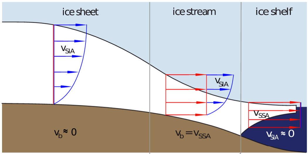
Figure 2: Superposition of Shallow Ice Approximation (blue arrows) and Shallow Shelf Approximation (red arrows) velocities in an ice sheet model. Schematic diagram of an ice profile showing different flow regimes, the arrow lengths represent how fast the ice flows, taken from M.A. Martin et. al., (2011): PISM – PIK – Part 2.

The model should be capable of solving the equations describing fast flow via parallel computations. We use the Shallow Shelf Approximation (SSA) to Stokes and solve the constant and transient version of these equations.
To account for ice-ocean interactions, the ice sheet model should have a melt-rate parametrization implemented (e.g., Seroussi et al., 2017).
You might want to code more than one sliding law (or different parameterizations of other physical processes that control the ice flow), to explore some of that structural uncertainty.

We can use our ice sheet model two ways: to solve (bake) an inverse problem and/or to solve a forward ice sheet problem. We are familiar with the concept of a forward problem; given a set of inputs, parameters, or initial conditions, we let the model estimate the ice sheet behaviour (ice velocities) and make projections of sea level – so, we look into the future of the ice sheet giving a set of initial conditions and inputs. Inverse problems are somewhat less familiar; given satellite ice velocity observations, we ask ourselves how did this data come about? What input parameters or initial conditions of the ice caused those ice velocity patterns shown in the satellite data? (see yellow box in Figure 1).

Don’t get confuse though, this is not about simulating the past, inverse problems are more like inferring the past, we work backwards from the observed data (e.g., satellite ice velocities) to determine an unknown caused, source or condition.

We want to design our ice sheet model so it solves the inverse problem first – i.e. find the unknown parameters that gave origin to the observations and estimate the initial state of the ice sheet/ice shelves for future (forward) simulations. In our baking recipe, we call these unknown parameters control parameters.

Don’t forget to define a quantity of interest (QoI) in the model; this will help examine how errors propagate from the observational data onto the QoI forecast and its uncertainty. For this recipe, the QoI is ice sheet mass loss or volume above floatation (which is equivalent to sea level rise). This QoI though, cannot be considered a realistic projection, as in this recipe we will use an idealised climate for the simulations, to make error quantification less complicated.

2.2 An Automatic Differentiation (AD) tool
The AD tool will efficiently and accurately compute derivatives of mathematical functions. Here, we use tlm_adjoint (Maddison et al., 2019) but there are other AD Python tools like pyadjoint. AD allows the model to efficiently calibrate control parameters via the minimization of a cost function (see Methods step 1, below).

2.3 A good discretization method
This involves choosing a good technique to convert continuous data (or variables) into discrete finite elements (e.g., Koziol et al., 2021), so the computer(s) can solve the complex ice flow Partial Differential Equations (PDEs), and capture the flow of ice streams (see Fig 2).

2.3 A computer cluster
We will need several nodes and lots of data storage for the simulations.

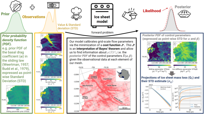
3. Baking terms explained (Bayes’ theorem)

Before getting into the actual recipe, we need to understand the meaning of Bayes’ theorem (Stuart, 2020) and how this is applied in the context of an ice sheet inverse problem:

In this equation:

p(X) is the Prior Probability Density Function (PDF) of our “hidden field” X. We cannot observe it directly – either because it is a hidden property under the ice (e.g., the basal drag coefficient) or because it is a large-scale property which in-situ experiments cannot reproduce. Yet we may have some preconception of how large or small this property can be or how it varies spatially – this is our “Prior” information; an “educated guess”, based on what we know/believe about this hidden property.

Imagine you are a chef creating a new pie, you start with a “prior recipe”, which is your best initial guess on how to make this pie taste amazing. However, you are open to adjust this recipe; as you get new feedback from your customers (i.e., as you get new evidence or information from the observations V). The process of adjusting the recipe with new information is what Bayes’ theorem is all about.

Here X is a function composed of two unknown parameter fields in the ice sheet model: the basal drag coefficient in the sliding law (noted as α) and a rheological parameter for describing ice stiffness (noted as β). If you are not familiar with these terms, check out this numerical modelling glossary.

p(V/X) is the likelihood function and represents the probability of observing the data (V) for a given sample of X. Among inverse modelers, this is known as the MAP (Maximum a Priori) estimate. It is also the mode (most likely parameter value) of the distribution that we seek.

p(V) is a normalization factor to ensure that the posterior PDF sums (or integrates) to one. Think of this as salt or sugar, it will always be part of our pie.

p(X|V) is the posterior probability density function (PDF) of X given the observational data (V), this represents our new improved pie recipe and ultimately what we want to bake: calibration uncertainty. The posterior represents our updated belief about the control parameters composing our hidden field (X) after incorporating the information gained by the observational data (V).

If X were just a number, or a few numbers and one parameter, this would be quite easy (like the upper diagram in Fig. 1). But because in our ice sheet problem this field is large (100,000 dimensions or more), we need another ingredient: a low-rank approximation to the posterior covariance matrix.

The posterior covariance matrix essentially describes the uncertainty in the control parameters (or hidden field) – this matrix is very, very large and is very hard to compute (even with a lot of computing power). However, via Automatic Differentiation, we can describe its mathematical inverse – and to find the covariance we need to only consider the parts of this matrix that are really determined by the model and observation data (Isaac et al., 2015). Our prior guess on the parameters will fill in the rest.

4. Ingredients (input data)

4.1 Observational data to calibrate model control parameters
For this recipe, we will use satellite ice velocities from ITS_LIVE for the year 2014 (Gardner et al., 2018, 2019)

4.2 Boundary conditions
Mask, topography, ice thickness, etc., comes from BedMachine v2.0.

4.3 Model domain
Here our model domain (red map in Fig. 1) is set up by generating an unstructured finite-element mesh using time-averaged strain rates computed from satellite velocity observations (MEaSUREs v1.0 1996–2012, Rignot et al., 2014). Strain rates represent how quickly ice deformations occur. The mesh resolution is highly heterogeneous and depends on the observed strain rates, we give the model more resolution (~ 200 m) to the parts of the domain that really need it (e.g., close to the calving front and in areas where velocities are higher; close to grounding line).

4.4 Prior Probability Density Function (prior PDF) of the control parameters

NOTE: This ingredient is a recipe on its own.
For the prior PDF of both control parameters (the basal drag coefficient in the sliding law α and a rheological parameter for describing ice stiffness β), we will need to make a first guess for their distribution (come up with our prior recipe).
We can do this by using L curve analysis, though be careful! This method has some limitations when it comes to error propagation; we explain this in the Section 4 of our paper, so check it out if you want more information.

If this is your first time baking (modelling), you might want to try different methods – so we encourage you to experiment with a different “prior recipe”. You can make informed guesses for the prior distribution based on the pointwise variance σ2 and auto-covariance length scale of each control parameter.
You can use this other method to find a prior, based on existing knowledge from the literature and the physical concepts that define each control parameters (see Recinos et. al., 2023 Section 4 for more information).

5. Step-by-step directions (the method)

STEP 1: Finding the MAP estimate

Let’s make use of our ice sheet model and our Automatic Differentiation tool, to solve the inverse problem and calibrate the control parameters. With this, we will find the initial state of the ice sheet given the model and the control parameters constrain by the observational data and the prior. This step outputs the parameter sets (the parameters spatial distributions of α and β) which give the best fit to ice velocity observations (Fig. 3).

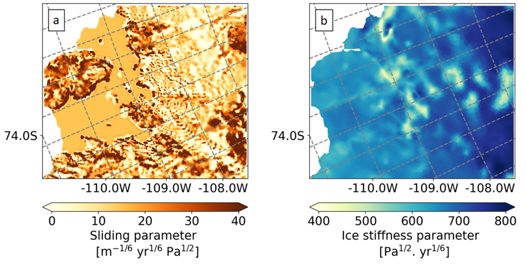
Figure 3: Inverted control parameters distributions (MAP estimates) for a) Basal drag coefficient (α) and b) Ice stiffness parameter (β). The velocity product used for this inversion is ITS_LIVE 2014. Images from and more information in Recinos, et al. 2023.

STEP 2: Use the calibrated model to make a projection of sea level change (the QoI)

Use the forward model to do what a forward model does! – That is calculate projections of the QoI with the parameters distributions from step 1 (parameters from Fig. 3).

STEP 3: Find how this projection varies as our control parameters change

This is a bit tricky and is where the Automatic Differentiation and our AD tool comes in hand. Using what is known as an adjoint method, we can see how our QoI will change for each tiny change in each one of our 100,000+ parameters.

Think of it as a very, very cheap sensitivity study. The output of this step should look like Fig 4.
The sensitivity maps in Fig 4. show that our QoI at year 40 (which is equivalent to projection of sea level change) is more sensitive to the control parameters at the grounding line.

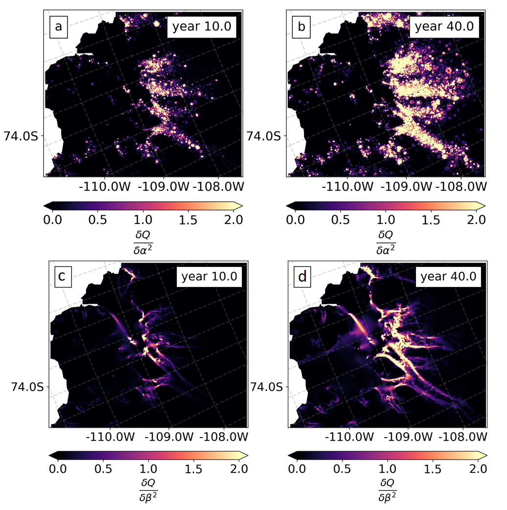
Figure 4: Sensitivity maps of the model’s change in volume above flotation (QT) in relation to changes to the basal traction α2 and the ice stiffness β2, for year 10 and year 40 of our simulation. Images from and more information in Recinos, et al. 2023.

Now, set this mixture aside in a bowl until it is ready to be used in the next step.

STEP 4: Approximate the posterior distribution of the control parameters.

Here we will use Bayes’ Theorem to update our knowledge of the control parameters using the observed data (we will update our prior recipe). The posterior distribution is quite a huge object and difficult to visualize (see Recinos, et al. 2023 section 5.1 for an example of how to visualize this) – and is only a preliminary step before we propagate this error into sea level rise projections – So let’s use our now improved posterior recipe for the final dish.

STEP 5: Use the outputs of Step 3 and 4 to see how uncertain our projected sea level is!
For our final step, we use the posterior distribution (our new recipe) and mix this with our adjoint sensitivities and voila! – we get an error estimate for sea level change. At least, considering calibration uncertainty (see Fig 5).

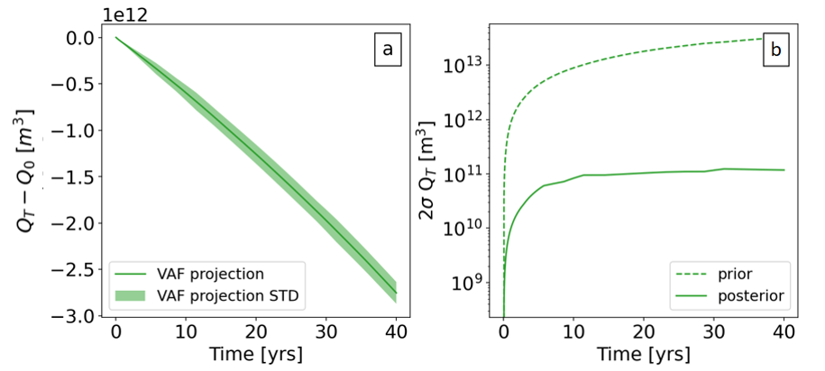
Figure 5: a) Solid green lines represents the trajectories of change in volume above floatation (which is equivalent to changes in sea level rise, i.e. QT -Q0) and the green shade its standard deviation estimate. b) Prior (dash lines) and posterior (solid line) uncertainty estimate of VAF over time (2σQT represents the 95 % confidence interval) [Credits Beatriz Recinos].

The uncertainty in the calibration parameters is good to know, but it is only the start, since ultimately we want to know and quantify all types of uncertainties in our projections.
However, calibration uncertainty does inform how likely sea level projections are. If our calibration parameters are random, then each random sample corresponds to a different sea level projection. Step 2, which says how projections change as parameters change, gives us a very fast way of quantifying this.
Remember, we use an idealized climate to generate projections of our QoI, and ideally, in the future we will implement realistic processes in this recipe, but also think of how we will quantify those errors when we bake the future of the ice sheet!
Providing meaningful probability estimates and improving how we communicate these estimates in our sea level rise projections is key to motivate decision-makers and stakeholders to use our projections.