Hidden beneath the surface of ice sheets lies an intricate structure carrying a unique fingerprint of past ice flow and climate conditions. Disentangling the drivers of an ice sheet’s enigmatic stratigraphy could theoretically unravel the ice sheet’s past evolution and provide a much clearer picture of things to come in the future. One way to detect this mysterious stratigraphy is to use ice-penetrating radars. Perhaps you have already come across these weird-stripy-fifty-shades-of-grey radar images? You know, radargramms… radargrammes…? Aah yes got it, radargrams! Well, keep on reading and we’ll take you on a little tour of the wealth of information that we can extract from the “stripes” visible on these radargrams, also known in the jargon as Internal Reflecting Horizons.
What are Internal Reflecting Horizons?
Internal Reflecting Horizons, a.k.a. IRHs, are bright reflectors found in the ice that can provide valuable information about past ice sheets processes (see Figure 1). Maybe you are asking “Reflector of what?”. Well, we are talking about the propagation of radar waves inside the ice, so the answer is radar waves! In the upper and middle part of the ice column, the presence of IRHs primarily depends on the variations in the density (as snow compacts into solid ice) and acidity of the ice (due to varying concentration of volcanic aerosols in the air at the time of snow deposition). These variations change the value of the dielectric permittivity of the snow/ice that the radar wave penetrates through.
Since waves reflect off of contrasts in dielectric permittivity, part of the wave is reflected back up, but because this contrast is small, part of the wave also keeps travelling down until it reaches the ice-bed interface, or otherwise just gets attenuated. Variations in density and acidity of snow and ice are typically related to snow and ice layers with a specific age. For this reason IRHs can be considered isochrones, i.e. their age is the same everywhere, and their distribution is a great tool to assess the age of ice inside of a glacier.
How bright an IRH appears on a radargram (radar image, Figure 1) will depend on how “different dielectrically” it is to the IRHs above and below. Because their brightness levels and continuity across radar profiles can vary, these IRHs can, in some places, be traced over large distances across the ice sheet (> 100 km), and in other places can only be traced for a few kilometres before they become too faint or too complex to follow. It is typically easier to trace them over the more slow-flowing regions of Antarctica or Greenland (see this study, this study, or this study) or in the more dynamic (i.e. faster-flowing) areas of the West Antarctic Ice Sheet (see this study or this study). This makes IRHs a very powerful complement to other past ice-sheet records such as ice or sediment cores, as they can provide a history of past ice-sheet dynamics over very large spatial areas.
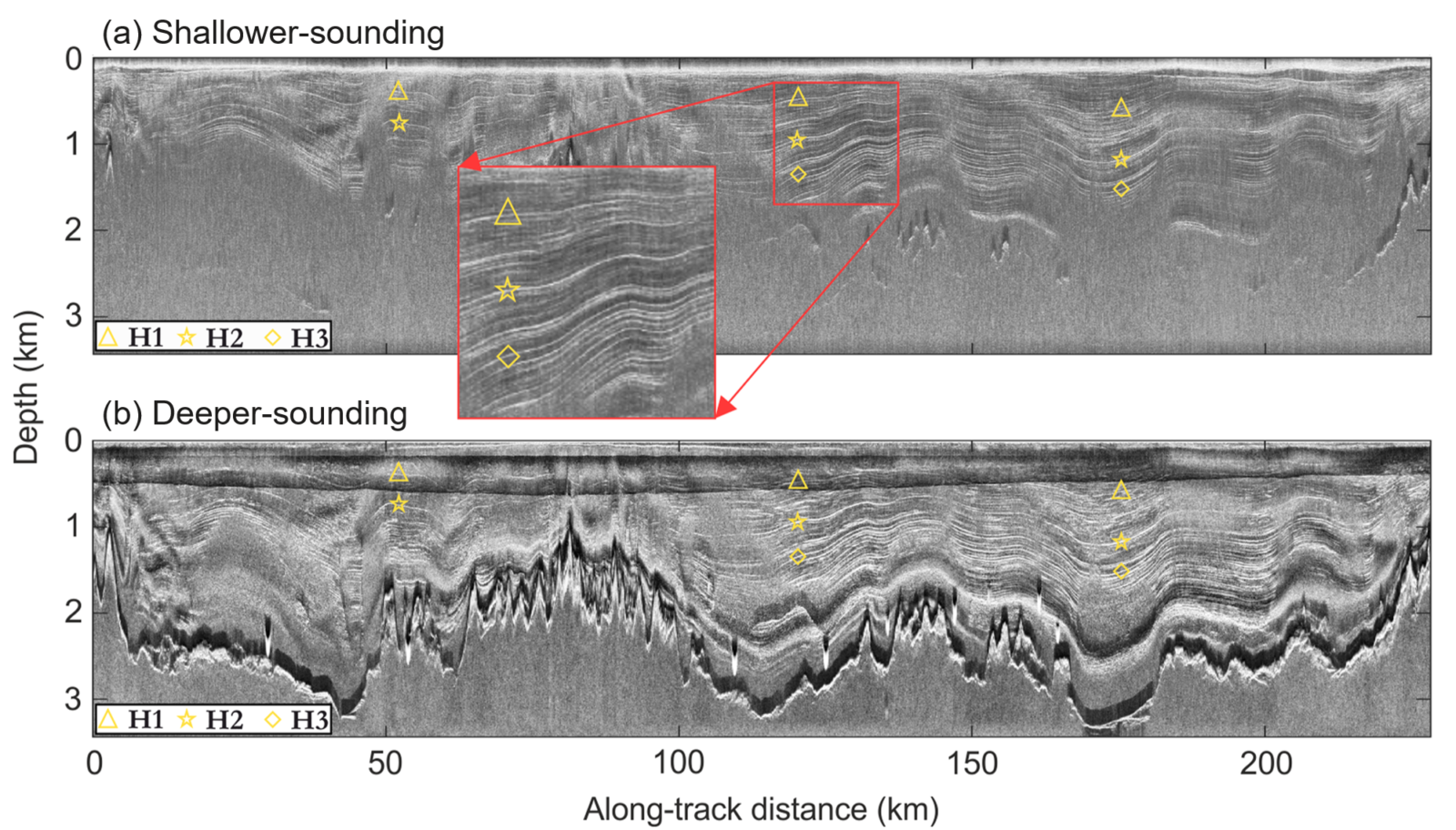
Example radargram from the British Antarctic Survey’s PASIN airborne radar system over Institute and Möller Ice Streams for (a) the shallower (upper 2-km in ice) and (b) deeper (up to 3 km in ice) radar modes. The yellow symbols represent three distinct IRHs widely seen across the catchment in the radar data. The inset in (a) shows a close-up look at those IRHs. In this figure, you can also see very clearly the ice-bed interface, where the bed appears very bright. Figure credit: Ashmore et al., 2020 (modified).
So, as mentioned above, IRHs can be considered layers of equal age, but how do we know the age of an individual layer? Well, that’s where ice cores come in! Where an IRH intersects an ice core site, it can be dated using the very accurate age-depth profile at the ice core. Depending on a large set of factors, including ice thickness, ice-flow speeds, the amount of melting at the bedrock interface, or the amount of snow accumulated each year, IRHs can be dated to as young as a few decades back (do you know how deep your birthday layer in Antarctica is?) or as old as several hundreds of millennia.
In addition, the number of IRHs that are visible on the data will depend on the frequency of the radar used: high frequencies (=short wavelength) lead to many thin IRHs that each represent fewer years, while low frequencies (=long wavelength) lead to thicker IRHs that each represent a longer time span. This is because the wavelength used will affect the pixel size in the radargram (i.e. the vertical resolution, and therefore the depth uncertainties; read on below). Quick technical note: high frequency radars are often referred to as “shallow” radars because the high frequencies get more quickly dissipated (i.e. lost) in the ice and can therefore only image the shallow portion of the ice column. Low frequency radars by contrast are often called “deep” radars because the signal can go all the way down to the ice-bedrock interface.
So, how can we use IRHs to infer past changes?
There are many ways that IRHs can be used to tell us about an ice-sheet’s history:
Understand past ice flow
IRHs (not necessarily dated) are useful to study past ice-flow dynamics such as speed and direction of ice flow. To do this, the geometries (i.e. shape) of the IRHs can be compared to current surface ice-flow velocities at the surface which we can measure with satellites.
Typically, IRHs start off at the surface as wide “flat” reflectors, which progressively get buried under successive snowfall events. The continuity of IRHs can be disrupted by ice dynamic effects leading to complex IRH geometries. This is typically seen in or near shear margins, when there is melting at the ice-bedrock interface, or where ice has to flow over subglacial mountains or troughs. A common method used to assess this is to compare the observed IRH geometries to modelled IRH geometries for unchanged flow in the past, and those differences can then be linked to historical flow changes!
Further down the ice column, fast-flowing ice can force ice crystals to align due to pressure and temperature changes of the ice. This can change the dielectric permittivity of the ice and therefore result in bright IRHs (this is what is referred to as anisotropy). Importantly, these IRHs are not isochrones, however their spatial distribution and orientation can still tell us a lot about past ice-flow history (read more about anisotropy in this previous Cryoblog post!).
Select future ice-core sites
Dated IRHs can also be used for ice-core site selection; in other words, they can help us decide where to drill a new ice core. Indeed, IRHs are very handy stratigraphic and age markers: bright and horizontal (i.e. undisturbed) IRHs in a particular location imply that drilling an ice core in that location would likely provide an ordered and intact climate record. For the Beyond EPICA Oldest Ice project, a project currently aiming at retrieving the oldest ice core ever drilled, the traced IRHs were used as input to a 1D model to predict the age of the ice below the deepest traced IRHs and find THE spot where 1.5 million-year-old ice could be retrieved (see a previous Cryoblog post on this here!).
Constrain ice sheet models
Dated IRHs are also starting to be used in large-scale ice-sheet models to answer the question of “how much & how fast will sea level change in the future?”
Indeed, the answer to this question is highly uncertain and tightly intertwined with the IRH stratigraphic records of Greenland and Antarctica. A sizable part (one might say the biggest part) of the uncertainties is due to the fact that current ice sheet models are operating on many parameters that are not so well-known or difficult to constrain. To limit their uncertainty, modellers compare their results with observations of current or past trends in ice sheet change. Undoubtedly, our knowledge on the contemporary evolution of the Antarctic and Greenland ice sheets has been propelled forward by the advent of scientific polar satellite observations. But unfortunately, this data is only available for the last couple of decades and usually limited to the surface characteristics of the ice sheet. As the evolution of an ice sheet and its response to changing climate conditions typically unfolds over centuries and millennia, the satellite record only provides a glimpse (albeit a tremendously valuable one) into the transient conditions of Greenland and Antarctica.
Thus, we need to go beyond the satellite record and provide a solid benchmark for models extending back in time. How? By integrating the depth and age of IRHs in ice sheet models! As these layers carry a unique fingerprint of all the relevant aspects governing ice flow (climate, internal deformation, basal melting/freezing even ice sheet instabilities), they are a treasure trove for ice sheet modellers. As the trove of traced and dated IRH’s of Antarctica and Greenland is steadily growing, this is a golden opportunity to take the next step towards fully calibrated ice sheet models (two first efforts to do so, here and here and even first jabs towards more complex modeling here!).
Quantify snowfall trends
Dated IRHs can also be used to infer past snow accumulation rates over large surface areas. This is important, as sea level rise can be slowed (albeit temporarily) if there is an increase in snow accumulation at the surface that is high enough to compensate for mass loss at the edge of ice sheets. Essentially, the amount of snow or ice accumulated between pairs of IRHs and the time period that it represents allows us to calculate a net accumulation rate. This is another useful constraint that model simulations can use to assess their skill: if the model simulations match past accumulation rate reconstructions, there is a higher chance they will correctly predict future changes, with important implications for estimating sea-level change.
Noteworthy are the shallow (high frequency) IRHs which, because of their high vertical resolution – often on the order of individual years – allow us to study the impact of climate change on accumulation rates. Using these shallow IRHs, we can also examine how homogenous, or rather how variable, snow accumulation is at the surface of the ice sheets (here and here are a few examples of studies). This is important to evaluate the mass balance of our ice sheets (i..e. their “health) because we usually rely on ice core records to provide observations of net yearly accumulation which are point-based while with radars we can get spatially distributed information.
So, if they are so important, surely we’ve already mapped them all, right?
Well, yes, but also, no! Over Greenland, IRHs have been traced successfully over most of the NASA Operation IceBridge airborne radar data (see this study and the embedded video), which covers a majority of the Greenland Ice Sheet.
Promotional video from NASA Operation IceBridge showing what we can learn from IRHs over the Greenland Ice Sheet. Video credit: NASA Goddard’s Scientific Visualization Studio.
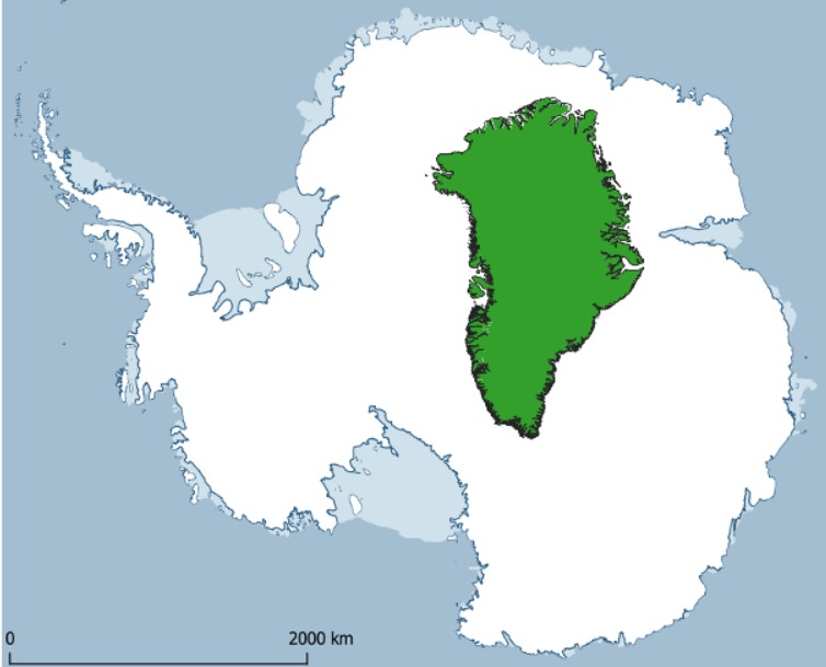
Figure2: Antarctica is about 7 times the size of Greenland (WGS 84 / Antarctic Polar Stereographic 71 S & WGS 84 / NSIDC Sea Ice Polar Stereographic North 70 N projections, prepared with Quantarctica and QGreenland). Figure credit: Brice Van Liefferinge.
However, over Antarctica, it’s a different task! Due to the sheer size and remoteness of Antarctica (almost 7 times the surface area of Greenland; Figure 2), it’s taking a lot more time to collect sufficient radar data to cover the whole continent. Only a handful of studies have managed to expand IRHs over large enough areas so far (see studies mentioned earlier here).
This is also due to the variety of institutes and data providers which collect radar data over Antarctica (see Figure 3), making data synthesis time consuming, in contrast to Greenland where most of this data is now publicly available from a single data provider.
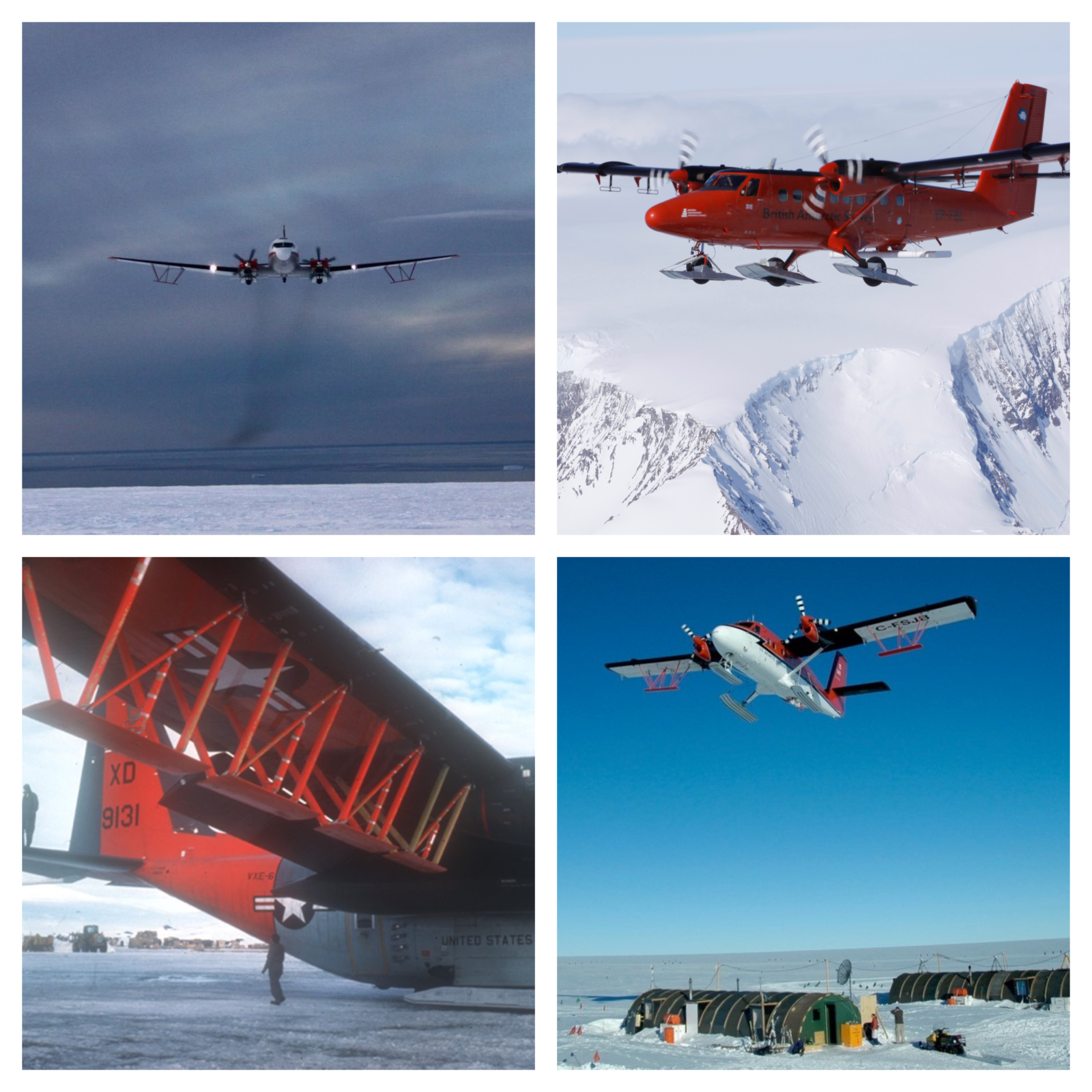
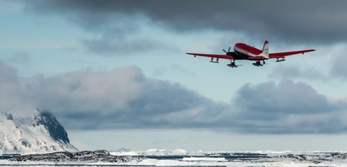
Figure 3: Photos of past and current aircrafts operating airborne radars over Antarctica. Note that these only represent a sample of all institutes and aircrafts operating ice-penetrating radars over Antarctica. For a fuller list, see Schroeder et al. (2020). From top left to bottom right: Basler aircraft flying over East Antarctica as part of the ICECAP 2008/09 survey using the University of Texas Institute for Geophysics (UTIG) HiCARS radar system (credit: Andrew Wright; shared by Martin Siegert); Twin-otter aircraft from the British Antarctic Survey operating the PASIN radar system over the Antarctic Peninsula (credit: Carl Robinson); United States C-130 aircraft used during the large-scale Antarctic radar surveys of the 1970s by the Scott Polar Institute-National Science Foundation-Technical University of Denmark collaboration (credit: Charles Swithinbank; shared by Martin Siegert); Twin-otter aircraft from Kenn Borek Air operating UTIG’s HiCARS radar system during the 2004/05 AGASEA survey of Thwaites Glacier (credit:Matt Fields-Johnson; shared by Duncan Young).
So, what’s next?
This is where the AntArchitecture effort comes in. AntArchitecture is a Scientific Committee on Antarctic Research (SCAR)-funded “action group” that aims to build an Antarctic-wide database of IRHs, and therefore obtain a complete age-depth model of the Antarctic Ice Sheet. This is already well underway, with many studies that have come out in recent years on the topic (see works cited here for some examples), however there is much more work to be done! This includes expanding the database of IRHs over most of East Antarctica and the Antarctic Peninsula.
In a similar way to the compilation effort of the BEDMAP project to collect all of Antarctica’s bed elevation data in one map, AntArchitecture aims to build a 3-dimensional view of the age and depth of the ice, so that this information can be used by modelling and observational studies of Antarctica.
To find out more about AntArchitecture and how to join, please visit the SCAR AntArchitecture website and subscribe to the mailing list for updates!
Further reading:
- Bingham & Siegert (2007) Radio-echo sounding over polar ice masses. Journal of Environmental and Engineering Geophysics 12:47-62.
- MacGregor et al. (2015) Radiostratigraphy and age structure of the Greenland Ice Sheet. J. Geophys. Res. Earth Surf. 120:212– 241.
- Plewes & Hubbard (2001) A review of the use of radio-echo sounding in glaciology. Progress in Physical Geography 25:203-236
- Siegert (1999) On the origin, nature and uses of Antarctic ice-sheet radio-echo layering. Progress in physical geography 23:159-179.
Edited by Giovanni Baccolo
 Julien Bodart is a final year PhD student at the University of Edinburgh’s School of GeoSciences and BAS. His research combines IRHs from airborne and ground-based radars together with modelled and observational atmospheric data to better understand past changes over West Antarctica. Julien is part of the SCAR AntArchitecture and BEDMAP3 groups, as well as the International Thwaites Glacier Collaboration GHOST team where he will conduct radar fieldwork in the 2022/23 Antarctic season. In his free time, he enjoys football, ice hockey, hiking, and kayaking. He sometimes tweets as @Julien_A_Bodart and can be contacted at julien.bodart@ed.ac.uk
 Marie Cavitte is currently a F.R.S.-FNRS postdoc at the Université catholique de Louvain-La-Neuve, in the Earth and Life Institute. She works on understanding the spatial variability of surface mass balance (net snow accumulation/ablation) at the interface between models and data. She never strays too far from her first love: radar data. Marie is part of the AntArchitecture and the RINGS SCAR Action Groups, the INSTANT Scientific Research Programme. Marie is one of the chief-editors of this blog! She tweets (too much) @MarieCavitte and you can email her at marie.cavitte@uclouvain.be.
 Johannes Sutter is based at the University of Bern as a research fellow of the German Research Foundation. He is pursuing an integration of isochrones into large scale ice sheet models to improve our understanding of past ice sheet dynamics and reduce model uncertainties. Johannes is also part of the AntArchitecture SCAR Action Group and interested in everything involving large chunks of flowing ice. You can reach him at johannes.sutter@unibe.ch.