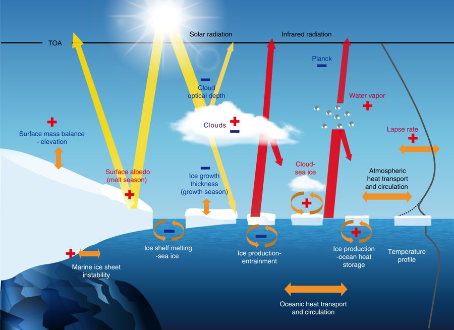
Figure 1: Major climate feedbacks operating in polar regions. Plus / minus signs mean that the feedbacks are positive / negative. Yellow and red arrows show solar shortwave and infrared radiation fluxes, respectively. Orange arrows show the flux exchanges between the different components of the climate system (ocean, atmosphere, ice) for several feedbacks. TOA refers to ‘top of the atmosphere’ [Credit: Fig 1 from Goosse et al. (2018)].
Over the recent decades, the Arctic has warmed twice as fast as the whole globe. This stronger warming, called “Arctic Amplification“, especially occurs in the Arctic because ice, ocean and atmosphere interact strongly, sometimes amplifying the warming, sometimes reducing it. These interactions are called “feedbacks” and are illustrated in our Image of the Week. Let’s see why these feedbacks are important, how we can measure them and what their implications are.
Climate feedbacks in polar regions
When it comes to climate science, feedback loops are very common. A climate feedback is a process that will either reinforce or diminish the effect of an initial perturbation in the climate system.
If the initial perturbation, for instance the warming of a region, is amplified by this process, we talk about a “positive feedback”. A positive feedback can be seen as a “vicious circle” as it will lead to an ever-ongoing amplification of the perturbation. The most prominent positive feedback in the Arctic is the “ice-albedo feedback“: as the surface warms, ice melts away, exposing darker surfaces to sunlight, which absorb more heat, leading to even more melting of the ice around.
On the contrary, if the initial perturbation is dampened by the process, we talk about a “negative feedback”. An example for a negative feedback is the “ice production-entrainment feedback”. In winter, when sea ice forms, it rejects salt into the ocean. As a result, the top ocean layer becomes denser and starts to sink. As the surface water sinks, it leaves room for warmer water below to rise to the surface. This warmer ocean surface then inhibits the formation of new sea ice.
The main climate feedbacks at play in polar regions involve the atmosphere, ocean and sea ice. They are represented in our Image of the Week. Plus and minus signs in this figure mean that the feedbacks are positive and negative, respectively.
How can we measure these feedbacks?
All the climate feedbacks depicted in our Image of the Week are far from being totally understood and are usually measured using different methods. That is why a new study (from which our Image of the Week is taken) proposes a common framework to quantify them.
In this framework, the feedback factor is the ratio between the changes due to the feedback only and the response of the full system including all feedbacks. It is positive for a positive feedback and negative for a negative feedback. In order to compute this feedback factor, we need to identify:
- the perturbation
- the reference variable involved in the feedback loop
- the full system, which includes all feedbacks
- the reference system in which the feedback under consideration does not operate.
If we take the example of the “ice production-entrainment feedback” (explained above):
- the perturbation is a given amount of sea-ice production
- the reference variable is sea-ice thickness
- the full system is sea ice and the ocean column with the entrainment process
- the reference system is sea ice and the ocean column without entrainment.
The feedback factor related to the “ice production-entrainment feedback” is then the ratio between the changes in ice thickness due to the feedback only and the total changes in ice thickness following a given amount of ice production. As it is a negative feedback, the related feedback factor is negative. As illustrated in Fig. 2, this feedback factor becomes even more negative, i.e. the strength of the feedback increases, with higher ice production. Therefore, this feedback is highly nonlinear, which is typical of feedbacks in polar regions.
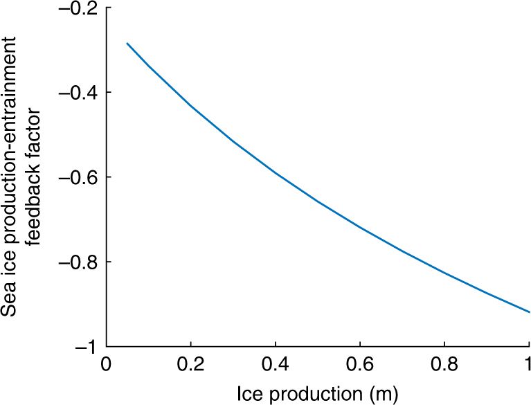
Figure 2: Feedback factor related to the ice production-entrainment feedback as a function of ice production. It is computed from mean temperature and salinity profiles in the Weddel Sea for January-February 1990-2005 [Credit: Fig. 5 from Goosse et al. (2018)].
The advantage of this framework is that you can apply it to all feedbacks present in our Image of the Week. Therefore, it is possible to compute their effects in a similar way, making the comparison easier.
Reducing uncertainties in model projections
Accounting for all those climate feedbacks is difficult, as they involve several components of the climate system and interactions between them. Therefore, their misrepresentation (or lack of representation) is one of the sources of error in model projections, i.e. climate model runs going up to 2100 and beyond. Climate feedbacks are therefore one explanation why models largely disagree when it comes to projecting global temperature and sea-ice evolution.
This means that, if we want to better predict what is going to happen in the polar regions, we must better measure what the feedbacks do in reality and better represent them in climate models.
On the modelling side, the main problem is that feedbacks are often described qualitatively to understand climate processes, and many models cannot evaluate these feedbacks quantitatively. There is therefore a clear motivation to use the common framework presented in this study to compute climate feedbacks in models.
However, additionally to improving model projections, identifying the critical climate feedbacks at play in polar regions is also a way to better target observational campaigns, such as the Year of Polar Prediction (YOPP) and the Multidisciplinary drifting Observatory for the Study of Arctic Climate (MOSAiC).
References
- Goosse, H. et al. (2018). Quantifying climate feedbacks in polar regions. Nature Communications, doi: 10.1038/s41467-018-04173-0.
- Pithan, F. and T. Mauritsen (2014). Arctic amplification dominated by temperature feedbacks in contemporary climate models. Nature Geoscience, doi: 10.1038/NGEO2071.
- Image of the Week – The warming effect of the decline of Arctic Sea Ice
- Image of the Week – Arctic changes in a warming climate
Edited by Sophie Berger and Clara Burgard
 David Docquier is a post-doctoral researcher at the Earth and Life Institute of Université catholique de Louvain (UCL) in Belgium. He works on the development of processed-based sea-ice metrics in order to improve the evaluation of global climate models (GCMs). His study is embedded within the EU Horizon 2020 PRIMAVERA project, which aims at developing a new generation of high-resolution GCMs to better represent the climate.