Earth’s surface is covered by many kinds of granular materials, including sediments and soils. Below ground, grains are also widespread in unconsolidated deposits and fault zones; even polycrystalline rocks deep inside the Earth are made up of mineral grains. These materials deform under their own weight and external forces, but what forces act inside them? In this blog post, we introduce experimental observations showing that some grains carry much stronger forces than others, together with a model that helps explain this inhomogeneous distribution. Why not take a closer look at how forces travel through granular materials—including familiar examples such as cereals and cosmetic powders?
Forces hidden inside granular materials
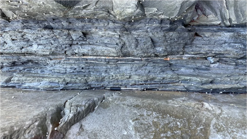
Granular materials, including unconsolidated sediments and soils, are widespread in the shallow Earth. Examples include surface soils, sedimentary layers and fault gouges (Fig. 1). These materials compact under their own weight and can undergo substantial deformation under external forces, such as tectonic stress. Their deformation is often modelled by treating them as a continuum, an approach that successfully explains many observations. Yet, inside a granular material, are the forces really distributed uniformly or smoothly? Forces within these materials drive deformation involved in sediment compaction, engineering operations that inject fluids underground, and fault movements that generate earthquakes.
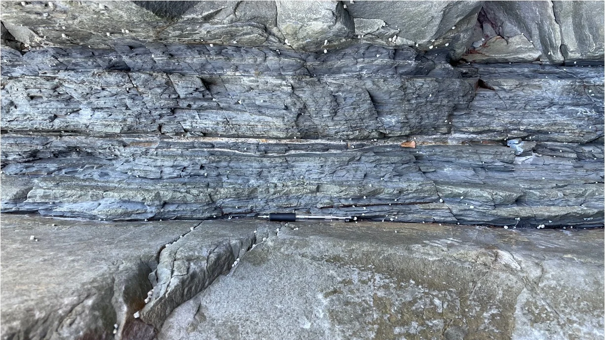
Figure 1. Example of shear localization in a mudstone layer within turbidites. Credits: Yuto Sasaki, 2026.
How do you think forces act inside a granular material?
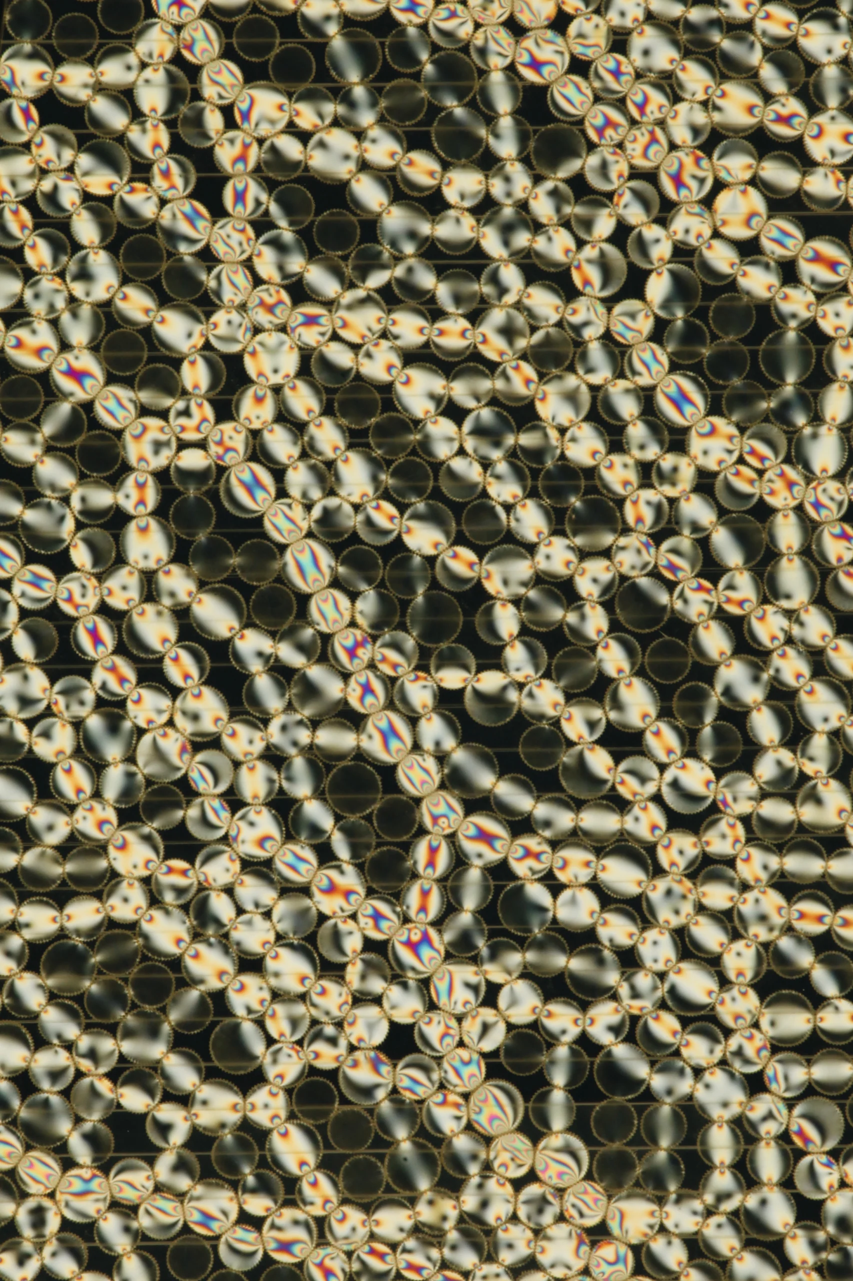
Figure 2. Force chains inside a granular material. Image: Aghil Abed Zadeh, CC BY 4.0, via Wikimedia.Commons.
Figure 2 visualises forces within a granular layer using a property called photoelasticity. The optical patterns reveal where the particles are strongly stressed. We can see that forces concentrate in some particles, forming a network of chain-like paths. Meanwhile, other particles carry much weaker forces. Looking more closely at a single particle, we find that it may transmit a strong force through its contact with one neighbour, while exchanging very little force with another.
How are the magnitudes of these forces distributed? Can we describe their distribution with an equation? Below, we introduce the essential ideas from Coppersmith et al. (1996). To give away the conclusion first, the model predicts that grains carrying very large loads are rare, as shown in Fig. 3. Experiments have also found a similar rapid decline in the frequency of large forces (Liu et al., 1995).
Now, let us focus on one grain within a layer of spherical particles under an external load. As shown in Fig. 4a, it receives forces from the surrounding particles through their contacts. Each arrow indicates a force exerted by the particle at its starting point on the particle at its endpoint. Forces are vectors, but, for simplicity, we consider their vertical components and take downward forces as positive. The positive forces from above balance the negative forces from below.
We can also view this balance as the transmission of force. Focusing on downward forces, the particle of interest receives a load from the particles above—and supports them through the equal and opposite reaction forces. It then applies the same total downward load to the particles below—and is supported by their reaction forces (Fig. 4b). Here, we neglect gravity. In reality, the magnitudes of the arrows in Fig. 4 vary considerably between contacts, and the total load received, or supported, also varies between grains. Finding the frequency distribution of this load is the aim of the second half of this post.
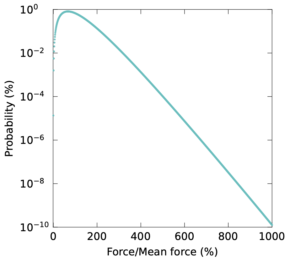
Figure 3. Probability density of the load supported by a particle, calculated from Eq. (7) with N = 3 (Coppersmith et al., 1996).
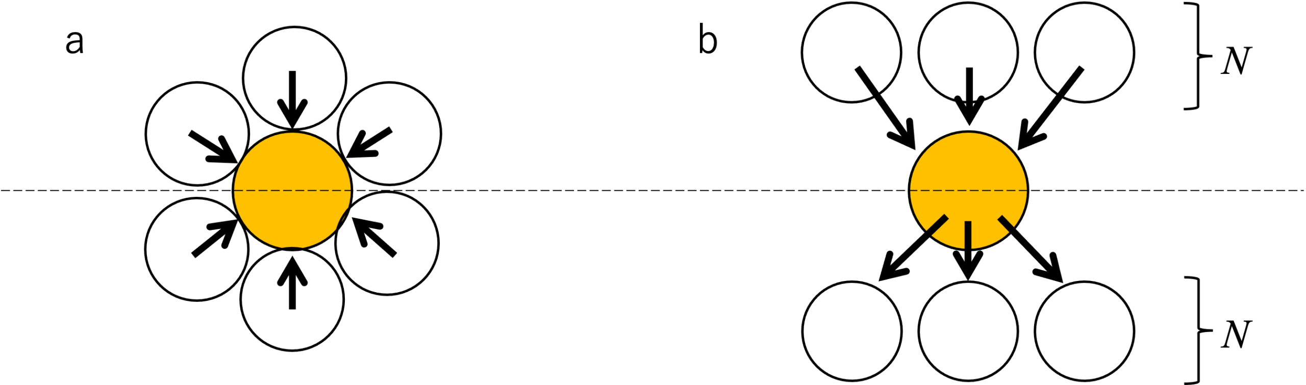
Figure 4. Model setup based on Coppersmith et al., 1996. (a) Particles in contact with each other. (b) N parent particles in the upper half apply positive force to the particle of interest (yellow), and the particle applies positive force to N child particles in the lower half (or the particle is subjected to negative force by N child particles).
What do we mean by a distribution?
Let us consider the stationary distribution of the load supported by each particle. In other words, we seek a distribution describing both the load on the particle of interest and the loads on the other particles that pass force to it. The individual values differ, but they should all follow the same distribution.
A distribution here means a probability distribution. For example, when we roll a fair die, each number from 1 to 6 has a probability of 1/6 (Fig. 5a). Unlike these separate outcomes, force can take continuous values. We therefore need to specify a range to assign a probability—for example, “the probability of a force greater than 2 N and no greater than 3 N is 1/6.”
For a constant density over that interval, the quantity that we multiply by the interval width, 3 − 2 = 1 N, to obtain the probability, 1/6, is called the probability density: here, 1/6 N−1. More generally, the probability is the area under the density curve across the interval. This is how we describe distributions of continuously varying quantities. Suppose, for example, that a force can take any value from 0.0 to 6.0 N, with the same density throughout. Its probability-density graph looks like Fig. 5b. Dividing the range into intervals of width 1 N gives six probabilities of 1/6, just like the bar heights in Fig. 5a.
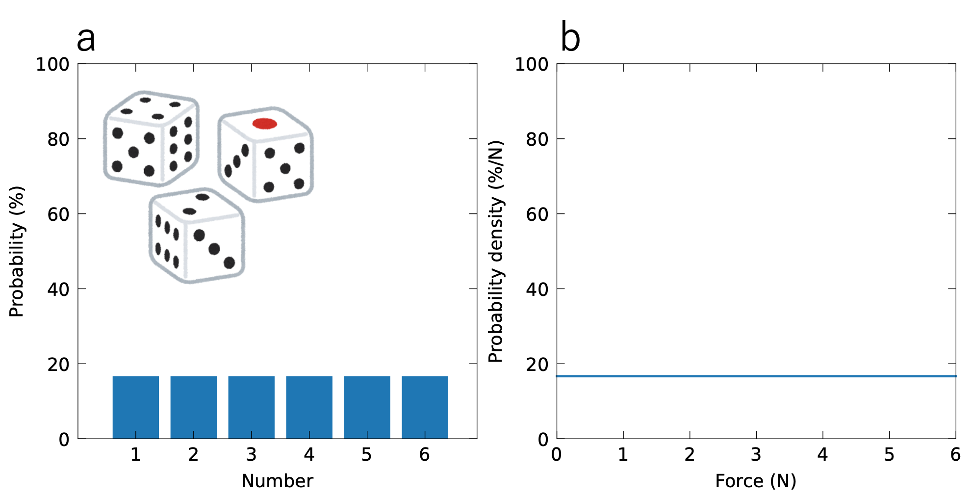
Figure 5. (a) Probability distribution of dice rolls. (b) Example of uniform probability density of continuous values.
How does one particle share its load?
Returning to the model in Fig. 4b, let us find the probability distribution (probability density) P(W) of the load W that the particle of interest supports—the total force received from above. A particle i in the upper half of Fig. 4b, which we call a “parent” particle, transmits a force xi to our “child” particle of interest. This is a fraction qi of the load wi supported by that parent: xi = qiwi . The fraction qi varies between 0 and 1. For any one parent, the fractions passed to all its children must add up to one. However, the fractions received by a child from different parents need not add up to one.
If the child receives forces from N parents, its total load is: W = x1 + x2 + … + xN = ∑i=1N xi . Many functions could be candidates for the probability distribution P(W). First, however, the mean-field argument for a model with genuine load splitting rules out a power-law tail proportional to W−α, where α is a positive constant. Intuitively, although splitting and combining forces can preserve the average load, it is difficult for an exceptionally large load to keep passing almost entirely from one particle to the next, with qi close to one each time. Mathematically, the moments—the averages of Wk—remain finite for all nonnegative integer k, whereas a power-law tail would make sufficiently high moments diverge. For the smooth tails considered here, this points to decay faster than any power law. At this stage, though, we know only that large loads are rare; we have not yet found the specific function.
The next step is to require the child-load probability P and the parent-load probability p to be the same function: P(W) = p(W), i.e., the stationary condition. The child’s load is the sum of the forces xi transmitted by its parents, and each transmitted force has some probability distribution F(x). Therefore,

In words, we multiply the probabilities for the incoming contributions, then add up all possible combinations of x1, x2, …, xN whose sum is W. This gives the probability distribution of the total load W on the child. For simplicity, we assume that the forces from different parents are independent and follow the same probability distribution F(x)—the mean-field approximation. In a real packing, however, the forces arriving from neighbouring parents may be correlated. To evaluate Equation (1), we need to know F(x).
Following the larger forces
How can we write the probability distribution of the force xi = qiwi transmitted by a parent? Let the probability distribution of the fraction be η(q), and assume that the fraction is independent of the parent’s load. Since w = x/q, the probability element can be written as: η(q) dq p(w) dw = η(q) p(x/q) (dq/q) dx . Integrating over all possible fractions gives,
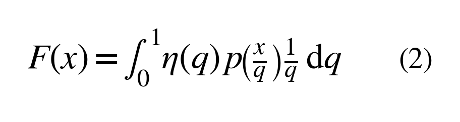
Now focus on the large-force end of the distribution. For a large transmitted force x, the main contribution to Equation (2) comes from fractions close to one, written as q = 1 − t, with t ≪ 1. A smaller fraction would require an even larger, rarer load on the parent. Like the child in Fig. 4b, each parent passes its load to N children. If one child receives the fraction 1 − t, the remaining N − 1 fractions of a parent must add up to t. Counting the possible allocations gives,
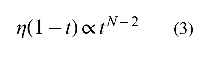
For small t, we assume that the possible ways of sharing the remaining fraction t have approximately the same probability distribution.
The other factor in Equation (2) is p(x/q). Since x/q = x/(1 − t) ≃ x + xt for small t, we can write log p(x/q) ≃ log p(x) − L(x)t. Here, L(w) is the negative slope of the log–log plot of p(w): L(w) = −d log p(w)/d log w = −w [d log p(w)/dw].
Thus, log[p(x + xt)/p(x)] ≃ −L(x)t, giving,

Substituting Equations (3) and (4) into Equation (2), using 1/q ≃ 1 in the region that dominates the integral, and collecting the proportionality factors into a constant C, we obtain,

In the final step, we used s = L(x)t. These steps describe the large-x approximation: the main contribution comes from small t. As discussed above, p(x) decays faster than any power law. Taking L(x) → ∞ as x → ∞, the remaining integral approaches a constant, giving:
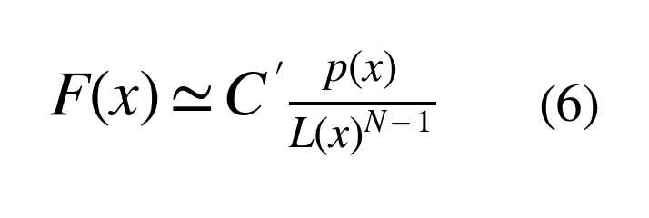
Here C′ is a proportionality constant independent of x.
A distribution that reproduces itself
Finally, substituting Equation (6) into Equation (1) lets us examine the large-load form of P(W). The parent probability distribution p appearing in Equation (6) and the child probability distribution P obtained from Equation (1) must be the same function. In other words, we need P(W)/p(W) = 1. Trying different forms leads to P(W) = C″(W) exp(−cW) under the assumptions above. A tail that decays faster or slower than this exponential does not reproduce itself. Here, C″(W) is not a constant; its large-W dependence is proportional to WN−1.
If this form holds over the whole range of loads, normalising it gives:

Here c is a positive constant. This whole-range expression is indeed a stationary solution when all allowed sets of outgoing fractions, adding up to one, are equally likely. For more general sharing rules satisfying the assumptions above, the argument above gives the large-load form proportional to WN−1exp(−cW), rather than fixing the entire curve.
To see the self-consistency, substitute p(w) ∝ wN−1 exp(−cw) into Equation (6). At large x, L(x) = cx − (N − 1) ≃ cx, so the powers of x cancel and F(x) ∝ exp(−cx). Substituting these exponential factors into Equation (1) makes the force-dependent part of the integrand particularly simple: exp(−cx1) exp(−cx2) exp(−cx3) … exp(−cxN) = exp[−c(x1 + x2 + … + xN)] = exp(−cW). It no longer depends on how the total force is divided between the incoming contributions. The integration supplies a factor proportional to WN−1, reproducing the same functional form.
Figure 3 shows Equation (7) for N = 3. Random packings of frictionless hard spheres in three dimensions have about six contacts per load-bearing particle (Silbert et al., 2002). This motivates the illustrative choice 2N = 6; the actual contact number depends on friction and packing conditions. The conclusion is that, in a model where contact forces split and combine, a small number of grains can carry loads several times greater than the average. Uneven force transmission is also visible spatially as the force-chain network in Fig. 2, although the load distribution alone does not determine the network’s arrangement.
This post introduces only the essential ideas; please see the original paper for the detailed arguments (Coppersmith et al., 1996). Later work explores further aspects of the problem. For example, contact forces xi should actually be vectors; the incoming forces have been treated as uncorrelated here, although neighbouring parents may carry correlated loads—a strongly loaded parent may have another strongly loaded parent nearby. The number of contacts also varies between grains.
Granular materials with such inhomogeneous internal forces are involved in many geological phenomena, including shear localization. Understanding their static and dynamic mechanical behaviour, and the statistical properties of their structure, therefore remains important. There is much more to discover about how microscopic arrangements of particles relate to the macroscopic behaviour of the materials beneath our feet.
References
Coppersmith, S. N., Liu, C.-h., Majumdar, S., Narayan, O. & Witten, T. A. (1996). Model for force fluctuations in bead packs. Physical Review E, 53, 4673–4685. https://doi.org/10.1103/PhysRevE.53.4673
Liu, C.-h., Nagel, S. R., Schecter, D. A., Coppersmith, S. N., Majumdar, S., Narayan, O. & Witten, T. A. (1995). Force fluctuations in bead packs. Science, 269, 513–515. https://doi.org/10.1126/science.269.5223.513
Silbert, L. E., Ertaş, D., Grest, G. S., Halsey, T. C. & Levine, D. (2002). Geometry of frictionless and frictional sphere packings. Physical Review E, 65, 031304. https://doi.org/10.1103/PhysRevE.65.031304
Abed Zadeh, A. (2017) Wikimedia Commons. https://commons.wikimedia.org/wiki/File:Force_chains_in_a_collection_of_particles.jpg