The question what drives tectonic plates has been around since plate tectonics was first developed. In principle, the fluid dynamics is well-known but what is not well known are the material properties, especially mantle viscosity structure which determines how much force is needed to pull a plate with a certain speed, but also how fast mantle convection, which may act as a driving force can occur. And while on a research cruise with the aim of better constraining mantle viscosity, we got a first-hand experience with another fluid dynamic system – the atmosphere. And this is what this story is about.
Why deploying so many instruments
First, for a bit of context, let’s go back to 2017: That summer I went for a research stay at the Earthquake Research Institute (ERI) of The University of Tokyo, and Kiyoshi Baba, a renowned expert on electromagnetic methods to study the mantle beneath oceans, explained me the idea he had for how oceanic upper mantle viscosity structure could be better constrained. This is illustrated in two cartoons: Until around 47 Ma, the Pacific plate moved approximately northward relative to the plume. Because of this northward plate motion and also overall northward mantle flow, a hot anomaly would have been emplaced approximately beneath the Emperor chain (Figure 1).
However, after around 47 Ma, plate motion shifted into a WNW direction, which would have sheared off the already emplaced material beneath the Emperor chain, and further material emanating from the Hawaiian plume that is still moved northward by large-scale mantle flow would have additionally been dragged westward by the plate (Figure 2). Where this anomalously hot material is located can be computed for different viscosity structures from both numerical and analytical models and by comparison with results obtained from an array of ocean bottom seismometers (OBS) and electromagnetometers (OBEM) one can then find out which viscosity structure is the most realistic. These instruments record seismic waves from distant earthquakes and electromagnetic variations, and hence can give indications on the seismic velocity and electric conductivity distribution in the mantle beneath, which, in combination, allow to estimate the temperature distribution.
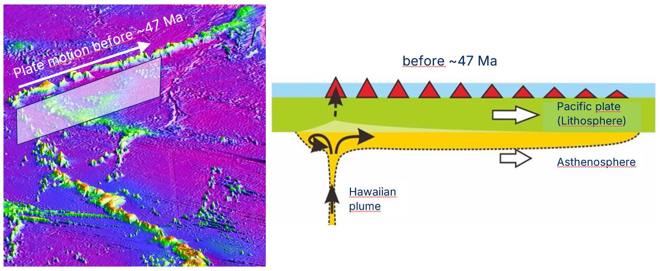
Figure 1: A hot anomaly is emplaced beneath the Emperor Chain by northward flow from the Hawaiian mantle plume, driven by plate motions and large-scale mantle flow. Credits: left: Bernhard Steinberger, produced with Generic Mapping Tools and Smith and Sandwell global topography dataset, right: Kiyoshi Baba.
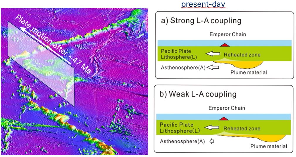
Figure 2: After a plate motion change around 47 Ma, the hot anomaly is sheared off from beneath the Emperor Chain while being replenished by continued northward mantle flow. Its expected position depends on how well it is coupled to the overlying plate. Credits: left: Bernhard Steinberger, produced with Generic Mapping Tools and Smith and Sandwell global topography dataset, right: Kiyoshi Baba
Let’s board the cruise
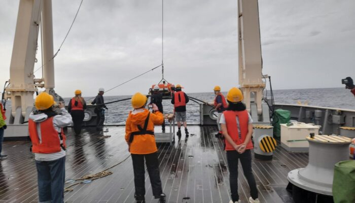
After successful proposals written by Kiyoshi Baba, Takehi Isse, Max Moorkamp, Marion Jegen , Antje Schlömer and myself, we obtained funding from Germany and Japan and after several years of waiting due to a backlog of cruises partly due to Covid we finally could get going: In October 2025 we deployed instruments (Figure 3) on board of the Japanese Research Vessel Hakuhomaru. Cruise participants came from a variety of institutions, including The University of Tokyo, JAMSTEC, Kobe University, Nagoya University, National Taiwan University, GEOMAR , AWI, TU Berlin, Uni München and GFZ to combine different areas of expertise (seismic and electromagnetic methods; geodynamic modelling) and reflecting from where instruments came from. The recovery cruise with the German research vessel Sonne is scheduled for spring 2026. Ideally, we would have liked a deployment for about 1 year, but because of scheduling issues this proved to be impossible (some Japanese instruments may stay longer, though, if the proposal for another Japanese cruise is funded).
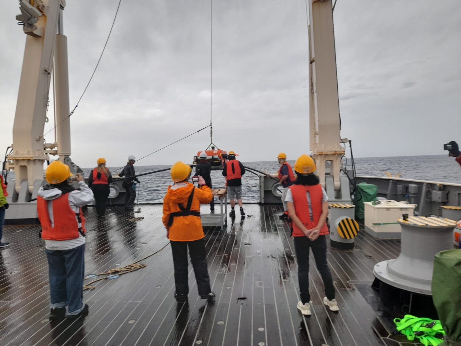
Figure 3: Deployment of an electromagnetometer (OBEM) from the institute GEOMAR. Photo by Bernhard Steinberger.
The plan
The area where the deployment was planned essentially targets where the western boundary of the temperature anomaly is modelled for different viscosity structures (Figure 4) and is shown in the first slide of figure 5. In the central part a closer instrument-spacing was planned, such that we get a higher resolution where we expect the boundary most likely to be. Additionally, we planned sites further out in order to cover a somewhat wider area and reach somewhat larger depth albeit with lower resolution. The planned station spacing was such that one could distinguish between the four models tested.
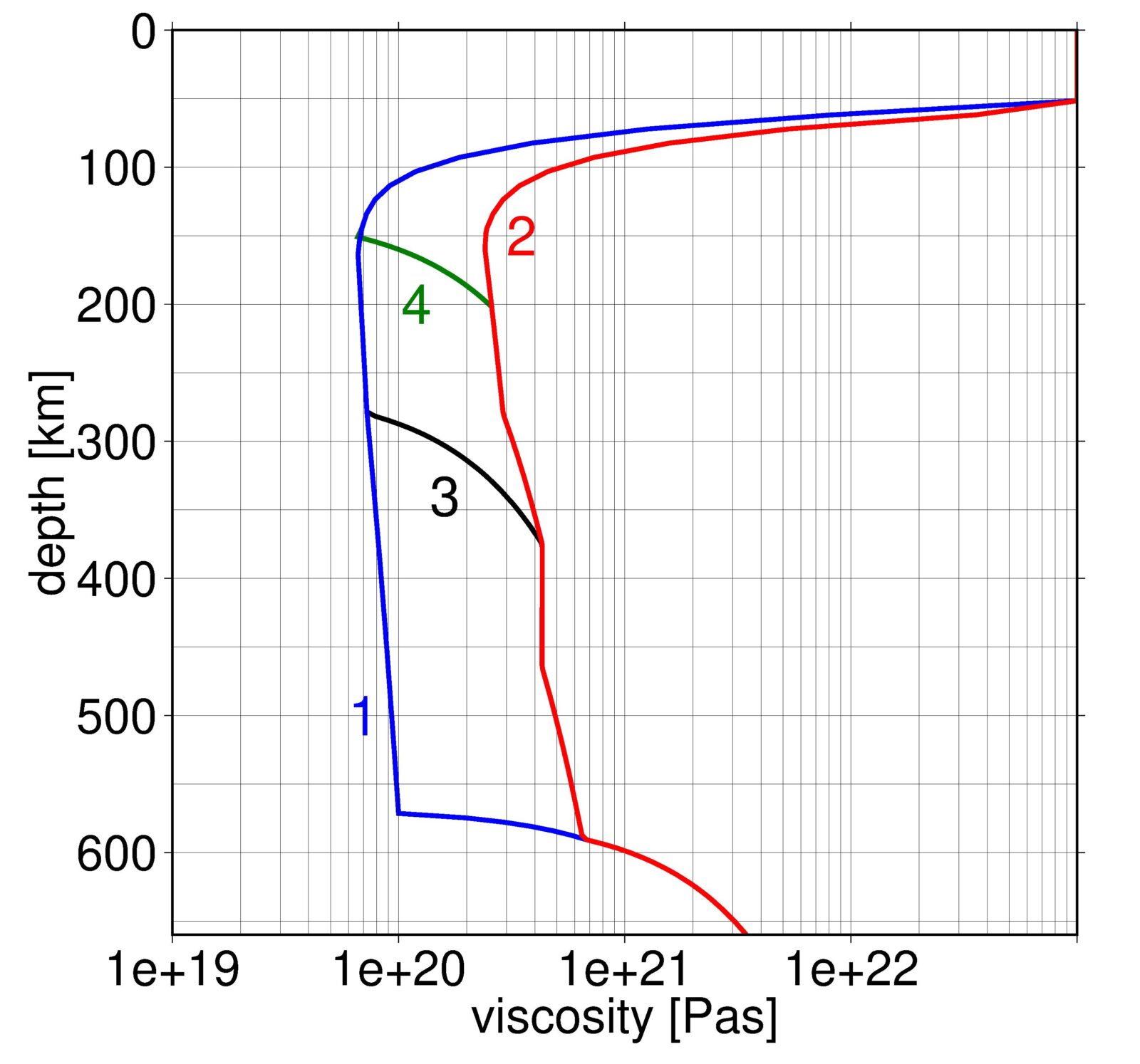
Figure 4: Four upper mantle viscosity models used in numerical models. The aim of the cruise is to collect data that can distinguish between these models. Figure produced by Bernhard Steinberger with Generic Mapping Tools
Changes of the plan and adaptation
High waves driven by bad weather and strong winds in the northern part of our field area made instrument deployment too risky, forcing us to change our plans several times. Decisions were made by the captain after consulting with chief scientist Kiyoshi Baba who himself consulted with other scientists participating in the cruise, aiming for the best scientific outcome that could be achieved under the constraints of weather and wave conditions. This loosing and gaining of ground is illustrated by a series of 18 slides in Figure 5. By cruise standards, though, this was a typical ride and I am not describing here an extraordinary adventure but the bread-and-butter reality of offshore sampling and research.
Figure 5: Video of the cruise plan. How the array changed with time. Thick blue, red, black and green lines labelled 1-4 show the western boundary (zero value of temperature anomaly relative to mean over the entire modelling area at 250 km depth) of a hot anomaly originating from the Hawaii plume, modelled with ASPECT (Heister et al. 2017) for four different viscosity models with the same color coding as in Figure 4. Background colors are temperature anomaly for the reference case (black line) with shades showing bathymetry above 3500 m depth – mainly Emperor Chain and Hess Rise – for orientation. Black dots indicate the sites we had been to and the grey-blue ship symbol the approximate ship location at the date indicated, green dots were the planned future sites. Credits: Bernhard Steinberger produced with Generic Mapping Tools
The first change of plans (slide 2) was to skip the north-eastern-most site at first and hope for better weather later on. This slightly modified plan was followed until Oct 6 (slide 3). Oct 7 never happened for us because we crossed the dateline that cuts right through the research area, but then conditions in the north still were windy with high waves for the foreseeable future so a more significant route change (slide 4) was decided on: We would gradually approach from south to north, still hoping the weather up north would eventually improve.
But around Oct 10 (slide5), the forecasts deteriorated for the entire remaining array, so we planned a slight change in the route (slide 6) that would allow us to escape to the southeast more quickly if the weather worsened any further. Unfortunately this really happened a day and three sites later (slide 7).
Hence the first painful decision had to be made; since there was no weather improvement foreseeable for the northernmost part of our array, we decided to abandon our plans to go there, and instead make the array denser in the southeast (“Plan B”, slide 8). We had only time to do deploy one more site (slide 9), before escaping to the southeast while we would do bathymetric surveys for three more sites where instruments were to be deployed later (that is why these sites were visited twice). These surveys were needed for most sites, in order to determine the exact deployment location because no maps of sufficient resolution existed. The surveys had the added value of being quite exciting, as we discovered many new features such as previously unknown seamounts (features that can often act as sort of oases in the abyssal plains, driving nutrient-rich water-upwellings and hosting a significant number of endemic species).
These provided further constraints on our deployment as the terrain should be reasonably flat in order for a deployment to be viable. In many cases, we had to shift the deployment site a few kilometers, because of newly discovered bathymetric features, from which we wanted to stay away, given that instruments may reach the ocean floor somewhat displaced relative to the release site due to ocean currents.
We expected to wait in our escape location near the southeastern corner of our array for about two days. However, about half a day later (slide 10), the forecast got slightly better such that it was decided to move to a somewhat more northerly position (slide 10 B), with the hope of finding a window of opportunity to go north after all. Nevertheless, the bad weather had already cost us so much time that we still had to abandon the northernmost sites. It turned out that we really only had to wait for a few hours, before a period of relatively calm conditions allowed us to cover some of those northeastern sites of our remaining array (slide 11 of Figure 5).
Unfortunately, on Oct 15 the forecasts worsened again, putting further sites out of our reaching (compare slides 11 and 12 of Figure 5). As an example for the kind of weather conditions we were facing, Figure 6 shows two storm systems north of our array. Since strong waves also radiate out from the storms, we had to maintain some distance to those to avoid high waves that would make deployment difficult or impossible. Hence, we had to change from overall “Plan B” abandoning the northernmost row of our array to “Plan C” abandoning two more rows. If we couldn’t go further north, we would at least try to make part of the array, where the boundary of the anomaly was most likely to be found, still denser. The hope to still go further north had not entirely vanished and indeed, less than a day later (slide 13) the improved weather forecast allowed for somewhat more optimism such that we scaled back on the dense central array again and first re-introduced stations in the north (slide 14) and after another day or so (slide 15) also in the west (slide 16) in our plan.
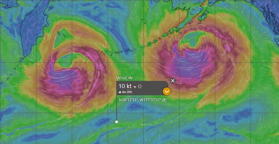
Figure 6: Position and wind conditions while at our northernmost site on Oct 20, 2025, 10 a.m. local time (UTC + 12). Windspeed 10 kt (knots) corresponds to a modest 18 km/hour at our location. Further north, winds were much stronger, also causing waves of several meters height with wavelength several tens to more than 100 m at our location. Figure produced with windy.com
By this time, we had had quite enough excitement and fortunately, we could follow this final plan laying out a well-rounded array with somewhat irregular spacing and slightly smaller and denser than originally planned, but nevertheless allowing for hope to achieve our goals. We think the final outcome was the best we could achieve given wind and wave conditions. No doubt the excitement will continue during the recovery cruise, where the rules of the game will be somewhat even tougher for us: We cannot just abandon sites unless we are willing to loose instruments.
References:
Heister, T., Dannberg, J., Gassmöller, R., & Bangerth, W. (2017). High accuracy mantle convection simulation through modern numerical methods – II: Realistic models and problems. Geophysical Journal International, 210 (2), 833–851.