Hello! My name is Erika Palmerio and I am a newly qualified Dr in space physics from the University of Helsinki, Finland. In this blog post I will talk about my PhD research and my future career plans.
The title of my PhD dissertation is “Magnetic structure and geoeffectiveness of coronal mass ejections”. Coronal mass ejections (or CMEs) are huge and spectacular clouds of magnetic field and plasma that regularly erupt from the Sun and travel throughout the heliosphere (that is, the region of space under the influence of our Sun). One of the most important reasons to study CMEs is that they are amongst the major drivers of what is known as space weather – a series of phenomena, disturbances, and technical failures that are caused by solar events. A number of these such effects are shown in Figure 1. CME-driven space weather effects on Earth (also known as geoeffectiveness) can range from satellite damages to beautiful aurora displays, including increased radiation to astronauts in orbit.
To better prepare and respond to the geoeffectiveness of CMEs, scientists are working to better understand and predict CME activity. Forecasting CMEs and their impact on Earth, however, is not as straightforward as it may seem. Firstly, as each CME is characterised by its own latitudinal and longitudinal extent, it is important to determine whether a CME will impact Earth at all (which is known as the hit/miss problem). Secondly, every CME has its own initial speed that will change by the time it reaches Earth because of interactions with the local solar wind speed (which is known as the arrival time problem). Finally, the direction of the magnetic fields within a CME plays an important role in driving space weather effects at Earth—the most geoeffective structures are those that are pointing southward of the ecliptic plane, because they interact the most with Earth’s intrinsic magnetic field, opening it to dangerous particles and radiation. This problem is known as the BZ problem (where Z indicates the north–south component).

Figure 1. Examples of ways in which space weather can affect Earth and its infrastructure. Image courtesy: ESA.
In order to be able to forecast the magnetic structure of CMEs, it is important to know how their magnetic fields are organised. CMEs erupt from the Sun as flux ropes, magnetic helical “tubes” that can be idealised into two main components: the axial field, which runs through the centre of the tube, and the helical field, which bends around the tube. Different combinations and orientations of these two fields yield different flux rope types, which are sketched in Figure 2. It is clear from Figure 2 that not all flux rope types contain southward field (denoted as “S”), hence the importance of knowing a priori the magnetic structure of an incoming CME.
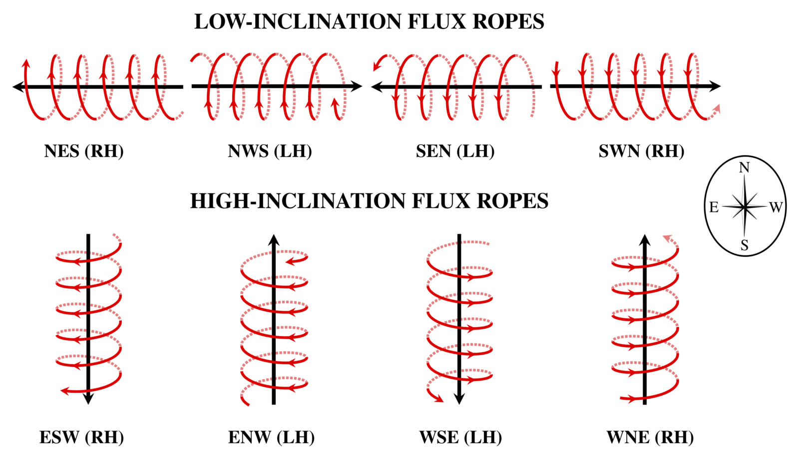
Figure 2. Combinations of axial (in black) and helical (in red) fields for the eight main flux rope types, where the low-inclination examples are parallel to the ecliptic plane and the high-inclination ones are perpendicular to it. The letters under each sketch represent the three field directions that a spacecraft will progressively encounter: the outer helical field, the axial field, and the inner helical field. “RH” means right-handed and “LH” means left-handed. The configurations of all other flux ropes can be considered as intermediate cases between these eight ideal states. The sketches shown here are compatible with the Geocentric Solar Ecliptic (GSE) and Geocentric Solar Magnetic (GSM) coordinate systems, where the east direction points roughly to the left when looking from Earth towards the Sun. Figure adapted from Palmerio et al. [2018].
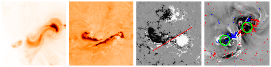
Figure 3. Examples of proxies from solar observations that can help identify the intrinsic flux rope type. From left to right: sigmoid (data: Hinode/XRT); flare ribbons (data: Hinode/SOT), polarity inversion line (in red) marked over magnetogram data (white = positive polarity, black = negative polarity; data: SDO/HMI); location of coronal dimmings (marked in green; data: SDO/AIA) with overlaid magnetogram data (red = positive polarity, blue = negative polarity; data: SDO/HMI). Note that these examples do not belong to the same event.
Once the intrinsic flux rope type has been determined, one would expect that the same flux rope type to be encountered at Earth. Unfortunately, this is not always the case. First of all, it is important to keep in mind that not all interplanetary CMEs (or ICMEs) show a flux rope configuration in in-situ spacecraft data. This may depend on interactions between CMEs and with the ambient solar wind, on local deformations of the whole CME body, and/or on the crossing location of a spacecraft with respect to the nose and central axis of a flux rope. The structure of ICMEs can be evaluated, for example, using magnetic field and plasma data that are collected in situ by spacecraft around Earth or elsewhere in the heliosphere. A CME that shows a flux rope configuration is also known as a magnetic cloud, whilst more complex configurations are known as complex ejecta. Examples of these two types of ICMEs are shown in Figure 4. A magnetic cloud is usually characterised by enhanced magnetic field magnitudes, a smooth rotation of the magnetic field direction over a large angle, and low temperatures. When the comparison of the flux rope type from the Sun to Earth is restricted to magnetic clouds only, the magnetic configuration is more or less retained in only 30% of the cases, with a few events mismatching by as much as 180° in the direction of the axial field. Whilst the chirality of flux ropes is maintained in all events (as expected, since magnetic helicity is a conserved quantity), their inclination and magnetic field direction may change drastically because of, for example, rotations of the whole CME body, the crossing location of the spacecraft along the flux rope tube, and/or local deformations of the CME. You can read a press release about these results on AGU’s Eos Research Spotlight here.
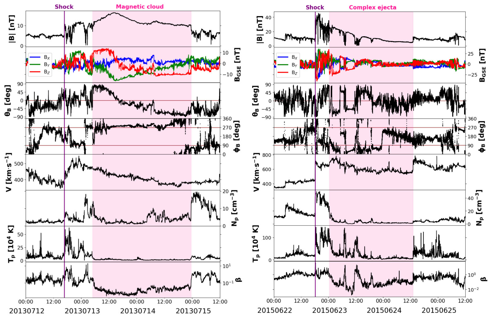
Figure 4. Examples of magnetic cloud (left) and complex ejecta (right). The parameters shown are, from top to bottom: magnetic field magnitude, magnetic field components in GSE cartesian coordinates, θ and φ angles of the magnetic field, solar wind speed, proton density, proton temperature, and plasma beta. The CME-driven shock is marked with a purple vertical line and the ICME ejecta is shaded in. Data are from the Wind spacecraft, located at Earth’s Lagrange L1 point.
The problems related to space weather forecasting of CMEs are not over yet! When CMEs are detected in situ, they are often accompanied by so-called interplanetary shocks ahead of them (as it is possible to notice in Figure 4). The region of shocked and compressed solar wind that lies between a shock and an ICME ejecta (flux-rope or not) is known as the sheath region. Sheath regions can be powerful drivers of geomagnetic storms themselves, but they are (if possible) even more challenging to forecast than CMEs, especially because of their turbulent and variable nature.
Two mechanisms that have been proposed to be responsible for the enhancement of magnetic fields that are pointing away from the ecliptic plane are the alignment of solar wind discontinuities downstream of interplanetary shocks and the draping of solar wind magnetic fields about ICME ejecta. These two mechanisms may result in planar magnetic structures (PMSs), which are periods in the solar wind where magnetic field vectors are highly variable in magnitude and direction, but nearly parallel to a single plane. A sketch showing the structure of a PMS, together with a so-called θ–φ diagram, is shown in Figure 5. The results of the analysis of about 100 sheath regions have shown that PMSs are present in most CME-driven sheaths, and they indeed seem to be associated with the strongest out-of-ecliptic fields (therefore, they seem to coincide with the most geoeffective parts of a sheath).
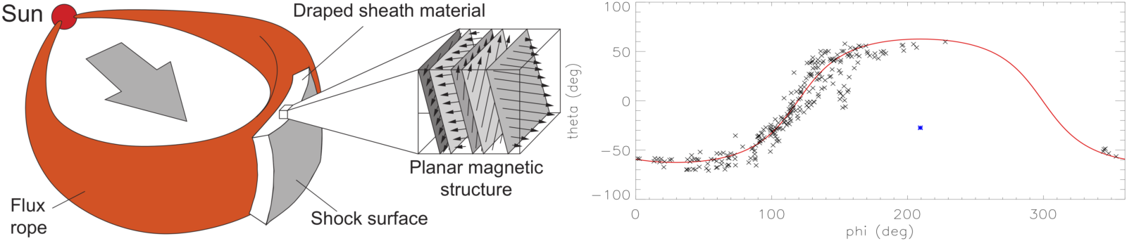
Figure 5. Left: Idealised representation of the formation of PMSs in the sheath regions ahead of CMEs. Figure reproduced from Kilpua et al. [2017]. Right: Example of a PMS visualised in a θ–φ diagram. Each black “x” symbol represents one data point in the sheath magnetic field, and the direction normal to the PMS plane (indicated by the red curve) is displayed by the blue star symbol. Figure reproduced from Palmerio et al. [2016].
Since forecasting multiple CME events is usually more complex than doing so for single CMEs, a useful tool for studying them is 3D heliospheric magnetohydrodynamics (MHD) modelling. The model that I have been using is called EUropean Heliospheric FORecasting Information Asset (EUHFORIA), which is developed as a joint effort between the University of Helsinki and KU Leuven. In the simplest configuration of EUHFORIA, CMEs are injected through the solar wind as hydrodynamic structures that lack an internal magnetic field configuration. These simulations have shown to be extremely useful in analysing where and when CMEs interact, but they do not allow studies of the resulting magnetic configuration unless the CMEs are launched as magnetised structures (which more recent EUHFORIA endeavours are devoted to). Nevertheless, coupling 3D heliospheric modelling with observational analyses and reconstructions can provide insightful information on the space weather effects of multiple and/or interacting CMEs.
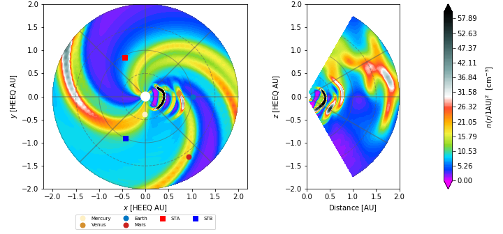
Figure 6. Example of three CMEs on their way towards Earth modelled with EUHFORIA [Pomoell and Poedts 2018] from the ecliptic plane (left) and from the meridional plane that contains Earth (right). Image courtesy: Eleanna Asvestari.
Palmerio, E.: Magnetic structure and geoeffectiveness of coronal mass ejections, University of Helsinki Report Series in Physics, D266, ISBN:978-951-51-2804-1, 2019.
Palmerio, E., Kilpua, E. K. J., and Savani, N. P.: Planar magnetic structures in coronal mass ejection-driven sheath regions, Annales Geophysicae, 34, 313–322, doi:10.5194/angeo-34-313-2016, 2016.
Palmerio, E., Kilpua, E. K. J., James, A. W., Green, L. M., Pomoell, J., Isavnin, A., and Valori, G.: Determining the intrinsic CME flux rope type using remote-sensing solar disk observations, Solar Physics, 292:39, doi:10.1007/s11207-017-1063-x, 2017.
Palmerio, E., Kilpua, E. K. J., Möstl, C., Bothmer, V., James, A. W., Green, L. M., Isavnin, A., Davies, J. A., and Harrison, R. A.: Coronal magnetic structure of earthbound CMEs and in situ comparison, Space Weather, 16, 442–460, doi:10.1002/2017SW001767, 2018.
Palmerio, E., Scolini, C., Barnes, D., Magdalenić, J., West, M. J., Zhukov, A. N., Rodriguez, L., Mierla, M., Good, S. W., Morosan, D. E., Kilpua, E. K. J., Pomoell, J., and Poedts, S.: Multipoint study of successive coronal mass ejections driving moderate disturbances at 1 au, The Astrophysical Journal, 878:37, doi:10.3847/1538-4357/ab1850, 2019.