The contribution from David Schlaphorst, the member of ECS SM division team. David is a PostDoc in Dom Luiz Institute (IDL), University of Lisbon, where he does seismology research.
Introduction
Distributed Acoustic Sensing (DAS) has been used exponentially over the last decade.If you are eager to learn the basics but in song form try this link.
In this blog post, we want to dive into one example of DAS recordings to show some different signals we can actually identify. This work was presented in a recent publication by Afonso Loureiro and co-authors (Loureiro et al., 2025; so far under review, preprint) and the following figures with their captions are all taken from that article. Also, there are many further interesting studies on DAS cables, focussing on all the different aspects in much more detail than what is shown in the following chapters or the paper itself, so follow the link to the paper to get the references of all those works. If you would like to learn more about the theory, follow this link to a previous blog post by SM ECS members Ana Nap and Katinka Tuinstra.
Location and Data
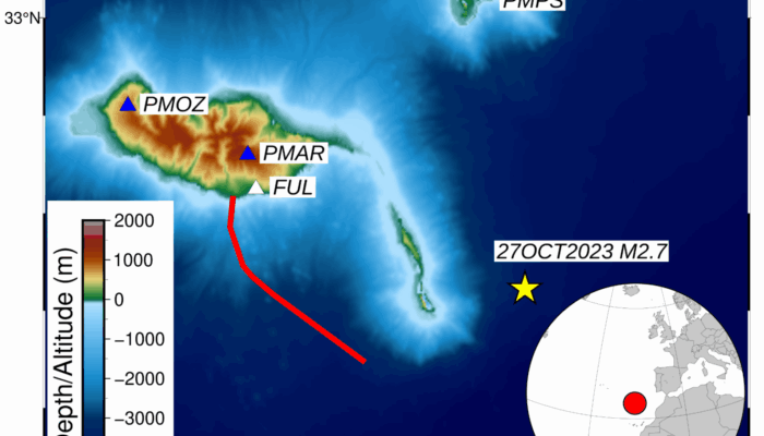
The data used in this work comes from a cable that has been deployed by EMACOM off the coast of the Portuguese island of Madeira in the Atlantic Ocean (Fig. 1) and runs for about 57 km. While the cable was installed for regular commercial traffic, one of the fibres in the cable (cables normally have multiple fibres) is a “dark fibre”, which means that it is only used for scientific purposes and does not interfere with regular communication traffic. ARDITI (Agência Regional para o Desenvolvimento da Investigação, Tecnologia e Inovação – regional agency for the development of investigation, technology and innovation) is responsible for the acquisition, maintenance and operation of the DAS interrogator. Even though recordings up to 2 kHz at a channel spacing of 1.02 m would be possible with the setup, it was decided to collect data at 500 Hz at a gauge length of 10.2 m (so, averaging 10 adjacent channels) with a 5.1 m spacing to have 50% overlap. This means that we have a recording of 500 Hz every 5.1 m over the entire length of 57 km. As you can imagine, this results in a staggering amount of data, roughly 1 TB per day, which immediately highlights one of the problems of DAS data recording and storage: one runs out of space to store the data quite fast!
The recording for scientific observations was started in late October of 2023 as part of the GeoLab initiative with the intention to provide free and accessible data to the scientific community. The work was done in as part of the Europe-wide multi-institutional project SUBMERSE. The present publication focuses on roughly one week of data during that initial phase (26/10/2023 to 03/11/2023).
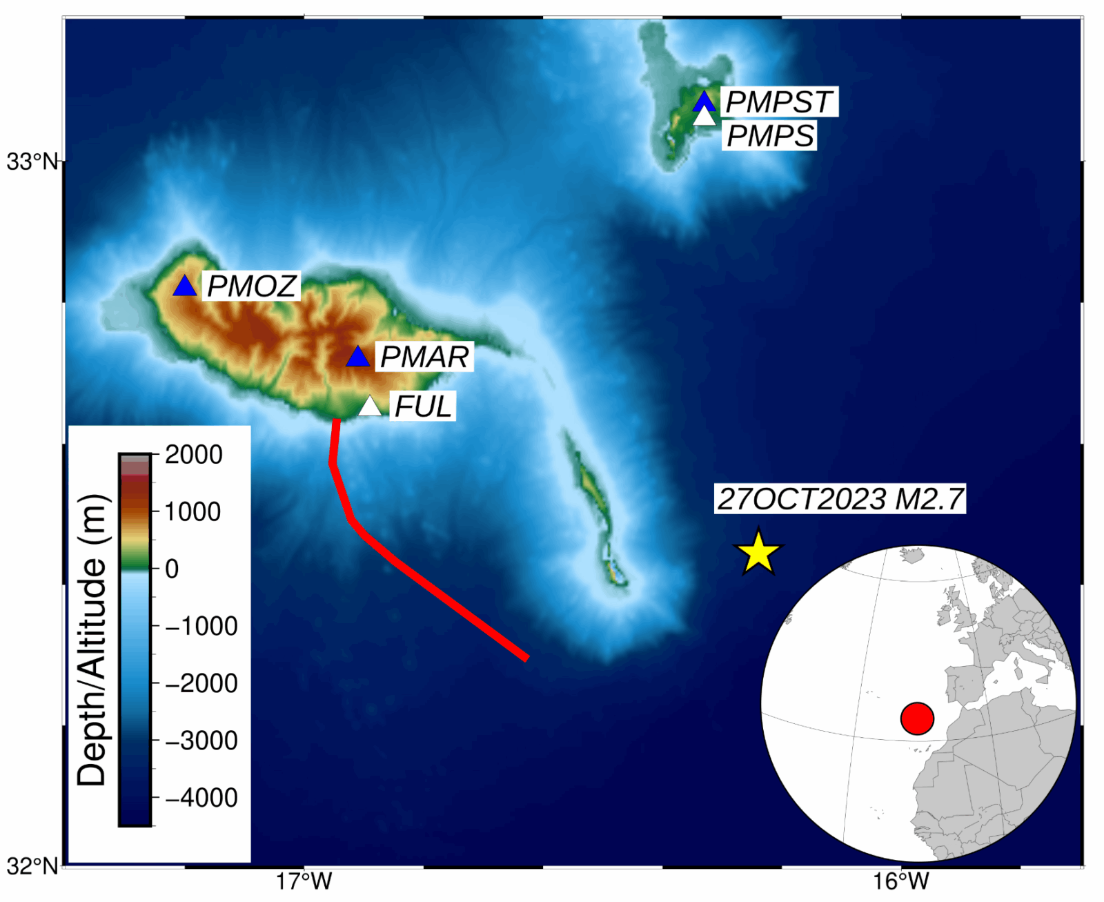
Fig. 1: Map of the Madeira archipelago, showing locations of the cable and permanent seismic stations. Red line: approximate location of the GeoLab fibre. Blue triangles: permanent broadband seismic stations. White triangles: permanent short-period seismic stations. Yellow star: local earthquake recorded during the data acquisition period. Topography and bathymetry source: GEBCO Compilation Group (2023).
Earthquake detection and T phases
Even though DAS cables only provide one component, marine deployments give us access to areas that we were previously unable to monitor with seismic stations, unless rather expensive OBS (ocean-bottom seismometer) experiments were carried out in the location. In addition, they provide them at an unprecedented spatial density. Because of this density, it is possible to easily recognise features that would be very hard or even impossible to observe with single seismic stations with a much lower density. For example, a recording of a local event (see the star in Fig. 1) gave not only the expected P and S phases, but also a T phase (Fig. 2). The T phase is generated when seismic energy is transmitted from the ground into the water column and kept there over sometimes very large distances in the SOFAR channel, a low velocity “valley” in the water where energy is channelled. Normally, T phases are not recorded this closely to the epicentre, but in this instance, due to the topography around the small islands between the event and the cable, seismic energy could be transmitted from the flanks of the islands into the water column and from there straight away to the cable.
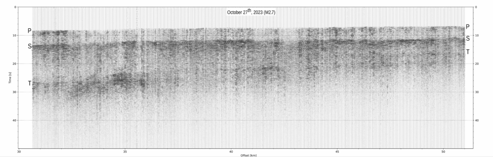
Fig. 2: Record section. Excerpt of a record section for the 27/10/2023 M 2.7 event. 125 m trace spacing. Band-passed between 0.5 Hz and 20 Hz.
Waves
Using a Fourier Transform on a part of the data (both in time and space, in our example it is a 30-minute interval on the first two marine kilometres) results in a plot in frequency-wavenumber space (f-k space; Fig. 3a). This is very useful, because surface waves show up here in distinct regions forming curves, also known as the dispersion curves. They can be calculated theoretically (see the dashed lines). However, the dispersion curves can get shifted in different ways and divert from that basic shape. For example, a current in the water along the cable can tilt both branches in land- or seaward direction. In addition, if the wave direction is at an oblique angle to the cable, a compression of both branches towards the middle vertical axis can happen. Checking the temporal variation of the curve can, therefore, give insight into changes in oceanic currents and wave directions. Using an f-k filter, it is possible to enhance directional signals and then focus on movement in only one direction along the cable. You can see that in Figs. 3b and c, after filtering only landward or seaward waves remain. The landward waves are much stronger, since the seaward waves almost exclusively consist of reflections at the coast.
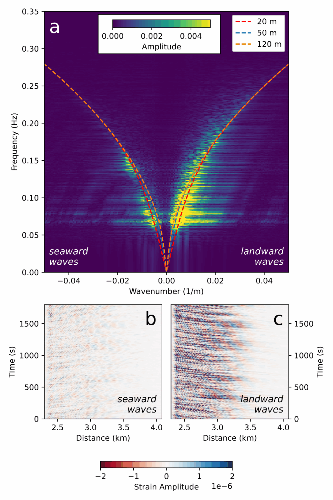
Fig. 3: Dispersion curves for the section of the cable subject to ocean waves. DAS recording over a 30-minute interval in the water close to the beach (start time: 27/10/2023 13:59:59 GMT; channels 450 to 800: ∼2.30 km to ∼4.09 km), bandpass filtered between 0.04 Hz and 0.35 Hz. a) Frequency-wavenumber spectrum. Theoretical dispersion curves without added currents are shown for water depths of 20 m, 50 m and 120 m, which covers the extent of the cable on those channels. Negative wavenumbers show the seaward direction of waves, and positive wavenumbers show the landward direction. b) Data after applying a directional f-k filter of 5 kms−1 to 50 kms−1, limiting the output to seaward waves. c) Data after applying the same f-k filter, but limiting the output to landward waves.
Tides
On the channels close to the coast, we can observe the change of the water column in roughly 12-hour cycles due to the influence of tides. Even though the actual tidal amplitude is less than 3 m, the effect can be traced to channels much further away from the shoreline. In fact, it is also possible to observe changes in wave directions and match those patterns to the tidal cycle.
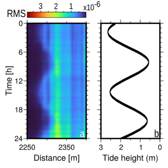
Fig. 4: Tidal imprint on the strain rate observed at the section of the cable entering the sea. a) root mean squared (RMS) calculated on 5 min windows between 2.25 km to 2.45 km cable distance for the first 24 h of recording. b) Tide heights calculated for Funchal. Note that the tidal amplitude is less than 3 m, but the signal of the waves hitting the beach is discernible along a ∼70 m slant distance.
Whales
Again, due to the dense channel spacing, it is quite easy to detect whale calls in the data, due to the distinct shape (see the hyperbola curves indicated by blue arrows in Fig. 5a) when looking at data filtered around the frequencies, in which the whales are expected to sing. Based on the position of these curves, we can determine the time and place of the whale. The vertex of the hyperbola gives us the position of the whale along the cable and the time, while the shape tells us about the distance to the cable. Whales can be detected up to a few tens of kilometres.
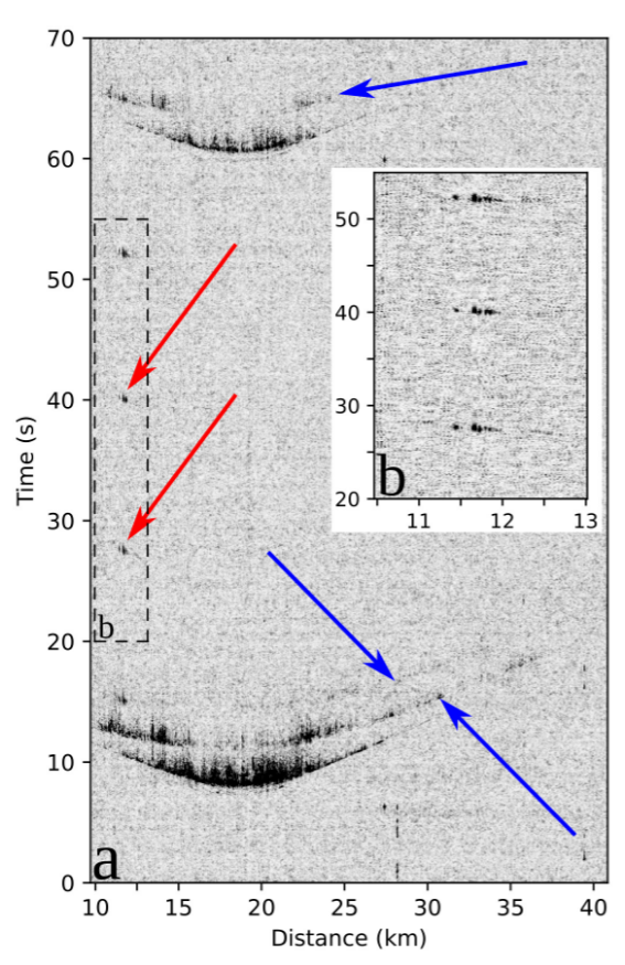
Fig. 5: Time-distance plot (start time: 29/10/2023 4:52:29 GMT). Data were filtered with an 8th order bandpass Butterworth filter between 12 Hz and 22 Hz, as well as an f-k filter to remove energy with an apparent velocity along the cable below 1.4 km/s. a) Multiple whale calls. At ∼11.7 km, the red arrows indicate fin whale 20 Hz calls with ∼13 s inter-note interval. Due to their distance, they are only detected on a small portion of the cable. A zoom of the region defined by the dashed line is shown in b). Blue arrows indicate multipath signals for the large hyperbolic events centred at ∼20 km. They are possible blue whale calls, but their origin is yet to be determined.
Having a closer look at a spectrogram can afterwards give us an indication of the species of whales, since whale calls vary among the different species (see examples of a sei whale and potential other biological signals in Figs. 6 and 7). These observations are incredibly valuable for studies on marine biology, since the monitoring of different whale species is complicated in the vast expanse of the oceans.
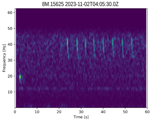
Fig. 6: Sei whale downsweeps. 60 s spectrogram of data from a channel at ∼15.6 km cable distance (start time: 02/11/2023 4:05:30 GMT). The single event at ∼20 Hz is a probable fin whale backbeat, although no downswept call is visible. To highlight the signal, data was filtered with an 8th order lowpass 50 Hz Butterworth filter.
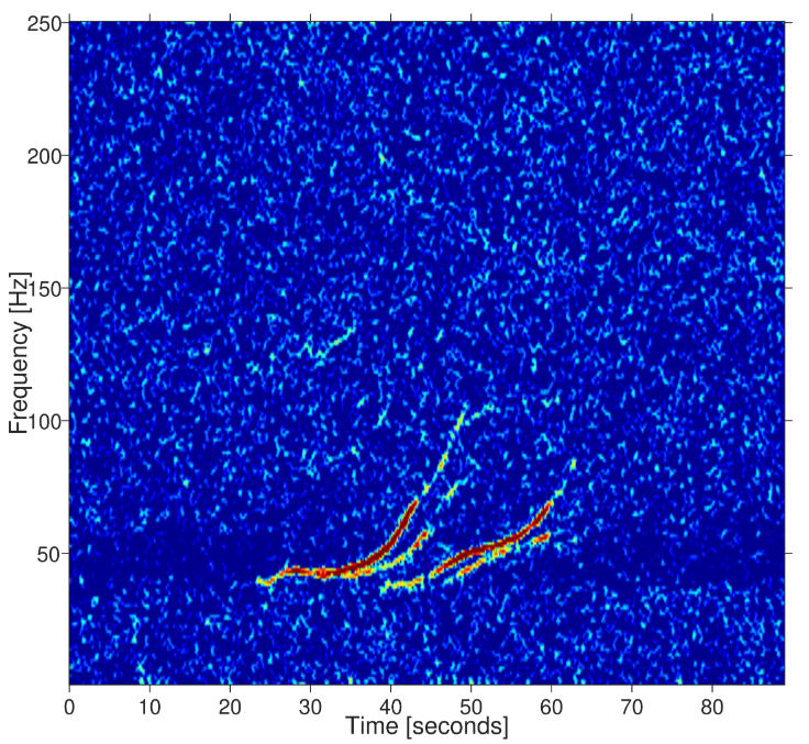
Fig. 7: Spectrogram of 90 s of data from a channel at ∼39.3 km cable distance starting at 2/11/2023 17:58:00 GMT, showing possible biological signals. Equalised by subtraction of the average noise levels.
Cars
This work focussed mainly on a marine DAS deployment. However, that does not mean that we cannot have a little bit of fun at times (well, and to show off more possibilities that exist with this deployment). The first two kilometres of the cable run on land next to some roads on Madeira before reaching the beach. On these sections, we can use DAS to map individual cars along the roads (Fig. 8a). That way, it is possible to see which drivers are going over the speed limit of the roads. What you can also see very well here is how the pattern in f-k space changes from the oceanic dispersion curves close to the coast to straight lines (Fig. 8b).
On top of that (and not mentioned in the paper, so you heard it here first!), we think we were able to spot buses of the local bus line and cross-checking with the timetables of those days could tell us that at least at one point the bus was late by 6 minutes.
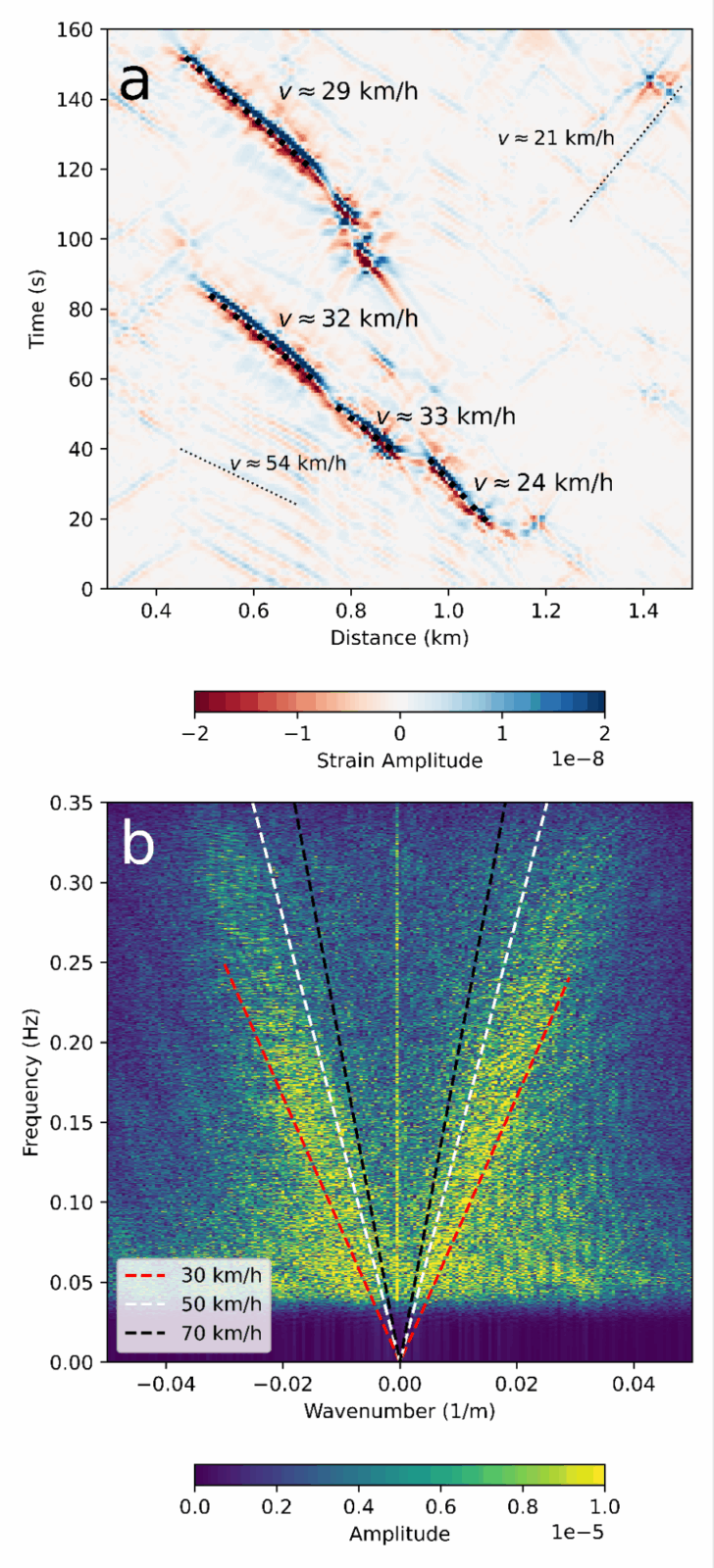
Fig. 8: Vehicles moving. DAS recording on land (start time: 27/10/2023 13:59:59 GMT). a) Subsection of 160 s, showing individual vehicles, as well as calculated velocities of a selection. b) Frequency-wavenumber spectrum of a 30-minute recording (channels 50 to 430 ∼0.25 km to ∼2.20 km), bandpass filtered between 0.04 Hz and 0.35 Hz. Constant velocities are shown as coloured dashed lines.
The Future is SMART
The previous chapters gave just a brief glimpse over some of the different features that can be observed, monitored and studied using DAS cables. Currently, scientific experiments are almost exclusively carried out on dark fibres and quite often those dark fibres only exist during limited time periods (for example because they are not in use during maintenance work). It is so far rare to have fibres continuously available for scientific research, like the one that was discussed here.
But on top of that, there are some exciting new developments in recent years, combining telecommunication with scientific instrumentation along its way, so called SMART cables (“Science Monitoring And Reliable Telecommunications”). The interesting part is that those additional instruments (for example seismometers, accelerometers, as well as pressure and temperature sensors) are included in the design of the cable already at the planning stage before deployment. Some initial tests have already been carried out, for example in the Mediterranean Sea in 2023 and very soon we will have the first larger-scale deployments, one 375 km section between Vanuatu and New Caledonia, and another 3,700 km cable connecting mainland Portugal with its archipelagos Madeira and the Azores. These installations are able to provide real-time data to greatly improve seismic and Tsunami early warning in those areas. If you are interested in more details, there is a very nice paper by Charlotte A. Rowe and co-authors (Rowe et al., 2022).
Hopefully, the overview of some of the many different features we can observe was interesting and maybe will even help you with your research. If you have any questions, don’t hesitate to contact us, we are always happy to chat about this research. There are obviously further observations that can be made and studies that can be carried out with such a cable, and that is why it is so exciting to have data available for free from this cable very shortly.
This work was funded by the Portuguese Fundação para a Ciência e a Tecnologia (FCT) I.P./MCTES through national funds (PIDDAC) – UIDB/50019/2020 (DOI: 10.54499/UIDB/50019/2020), UIDP/50019/2020 (DOI: 10.54499/UIDP/50019/2020) and LA/P/0068/2020 (DOI: 10.54499/LA/P/0068/2020), by the MODAS project 2022.02359.PTDC and by EC project SUBMERSE, HORIZON-INFRA-2022-TECH-01-101095055.