In this blog we give a succinct introduction to Distributed Acoustic Sensing for the starting seismologist, or the interested reader. The blog is by no means a complete overview and serves as a starting point for you to understand DAS and get started with the data. It was written by SM ECS members Ana Nap and Katinka Tuinstra.
By now, Distributed Acoustic Sensing (DAS) is a pretty widely known term among the seismological community. This measurement technique, which started emerging around 2010, has grown exponentially since then, as can be seen in Figure 1.
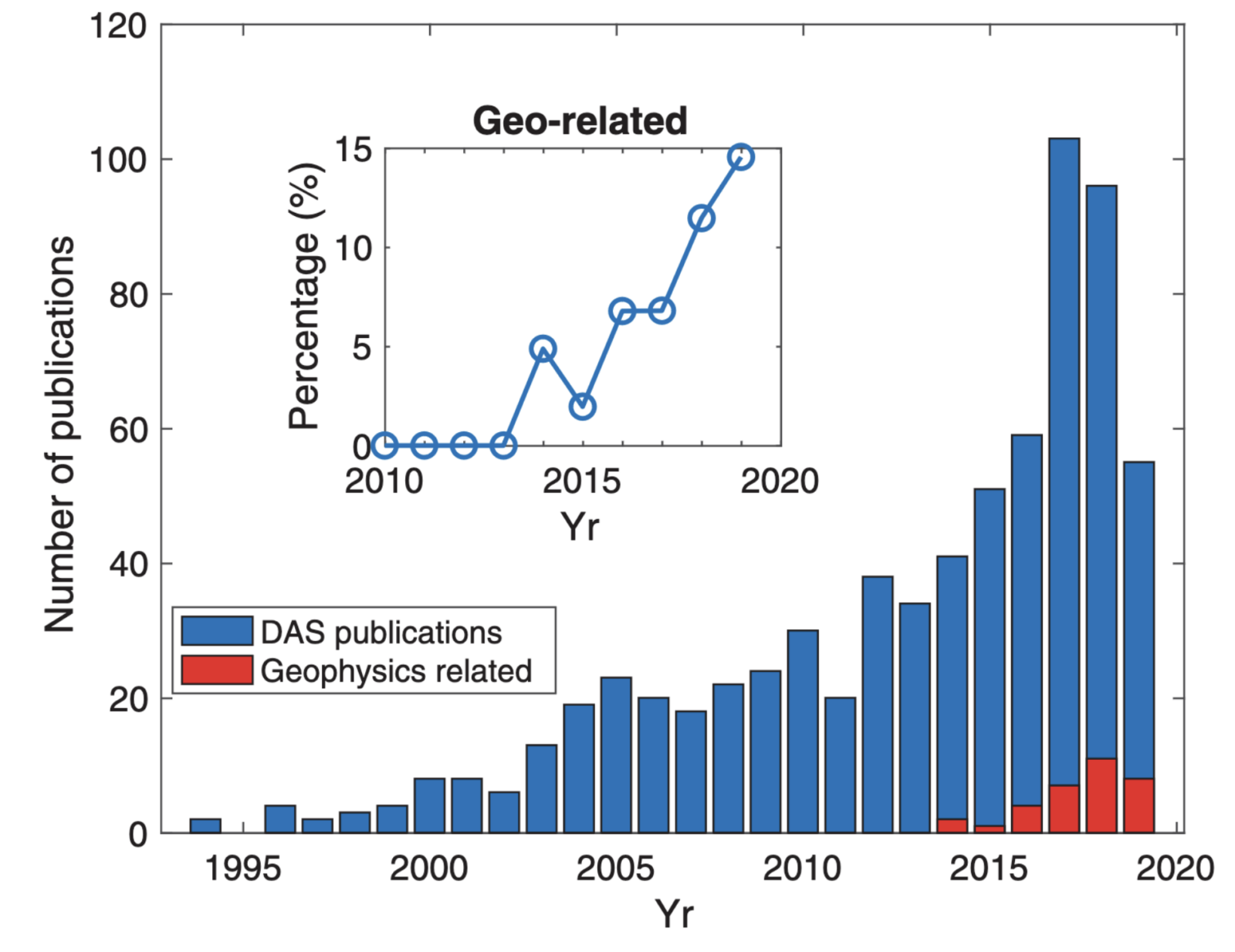
Figure 1: “Trend of publications related to Distributed Acoustic Sensing, according to the Web of Science (data accessed in July 2019).” Zhan, Z. (2019). Although this figure is from before 2020, it clearly shows the exponential growth in DAS research since the early 2000s.
While numerous seismologists may already be familiar with DAS and approximately know how it works, we still think people are looking for (extra) information. This blog is for the seismologists who have been living under a rock, the geoscientists who are new to seismology (or specifically new to DAS), and the people who have heard about DAS but remain unsure about what it is and how it works. We are here to assist all those people, to answer that burning question of “What actually is DAS?” and “How does it work?!” and once and for all provide them with this essential information.
So what actually is DAS? The short explanation
Distributed Acoustic Sensing (DAS) is a measurement technique that uses fiber-optic cables (such as those that are connecting you to the internet in many places of the world!) as a sensor for strain or strain-rate along the fiber-optic cable. When, for example, an earthquake reaches the cable, the fiber is stretched and compressed by the seismic waves i.e. strain of the cable.
It employs a (very fancy) laser in an interrogator unit (basically an expensive black box), that is connected to the fiber-optic cable, to shoot finite laser pulses into the fiber. Due to natural imperfections of the cable, part of the laser light is backscattered towards the interrogator. The interrogator can analyze this backscattered signal and translate this to strain or strain-rate along the cable. The spatial intervals of the measurement points can be from 10s of meters down to 20 cm depending on your use case. (The next section provides a more detailed explanation of the measuring method).
The main benefits of DAS lie in this vast number of measurement points, the broad range of frequencies that can be measured, the relatively low cost, and the relative ease of deployment of these cables in certain challenging environments (such as boreholes for example.)
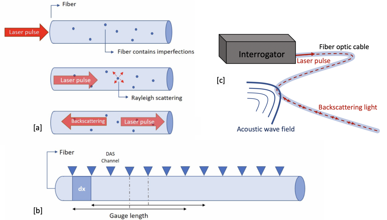
Figure 2: [a] Schematic drawing of the measuring principle of DAS. A laser pulse is sent into the cable from the interrogator, and due to naturally occurring inhomogeneities, Rayleigh scattering occurs. Part of this scattered light is backscattering towards the start of the cable (where the interrogator is attached, see [c]). [b] Strain or strain-rate of each DAS channel, spaced by dx, is determined across a gauge length which works like a moving average across the fiber optic cable. [c] When strain occurs in the fiber optic cable due to acoustic waves, the signal of the backscattering light that reaches the interrogator changes. From these changes, the interrogator calculates the strain or strain-rate occurring in the cable for each DAS channel. The figure is not to scale. Adapted from Nap (2020).
A more detailed explanation
The backscattering of the laser pulse light occurs due to naturally occurring inhomogeneities (density anomalies) in the fiber that are smaller than the wavelength of light. These anomalies produce light scattering within the fiber (specifically Rayleigh scattering). Part of this scattering is backscattering towards the start of the fiber attached to the interrogator (see Figure 1). The DAS interrogator analyzes the phase information of the backscattered signal. Simply put, if strain occurs in the fiber (due to seismic waves for example), the phase of the backscattered signal originating from approximately the same location will change. By analyzing the change in phase between the backscattered signals the strain can be derived. The word “Distributed” stands for the fact that with DAS, you are not measuring the phase change of exactly each channel, a channel is the midpoint of a moving averaging operation called a “gauge length”, which has a fixed length and is tied to the length of the light pulse. For all channels, separated by a set channel spacing of dx, the strain is determined across this gauge length. The relation between the gauge length, the separate channels, and the spatial sampling dx can be found in Figure 1b. The gauge length in many interrogators is set at 10 m, but this can be different depending on the brand of the interrogator and the settings. The exact location of a channel within its gauge length is unknown but is approximated to be in the middle. After setting up your cable and your desired spatial settings, channel location can be most accurately approximated by doing a tap test along the cable (literally going along the cable and tapping it by hand at certain points). This allows you to observe in the raw data which channel number corresponds to the location of the tap test on the cable.
Do you want to dive even further into the theory? Here are some examples of books and articles to start:
- Lindsey, N. J., Rademacher, H., & Ajo-Franklin, J. B. (2020). On the broadband instrument response of fiber-optic DAS arrays. Journal of Geophysical Research: Solid Earth, 125, e2019JB018145.
- Zhongwen Zhan; Distributed Acoustic Sensing Turns Fiber‐Optic Cables into Sensitive Seismic Antennas. Seismological Research Letters 2019; 91 (1): 1–15.
Some challenges
There are still some challenges with fiber-optic measurement techniques. For example, if they lie in a straight line, it only measures the strain along the fiber, so the data will be one component. Fiber deployment seems easy, but can still come with significant challenges to actually couple the cable to the medium you’re trying to measure, and fiber is quite fragile so it should be handled with care. Another challenge is in the data volume: DAS makes beautiful pictures, but at the cost of huge data volumes too! If you really exploit the maximum recording settings, the data could amount to up to TeraBytes per day. But in these challenges lies the fun: many researchers are at work to tackle these challenges, and integrate DAS into monitoring networks.
What does DAS data look like?
Enough theory for now! What does the data look like? Let’s start with an earthquake that was recorded on two pieces of fiber:
Earthquake DAS data
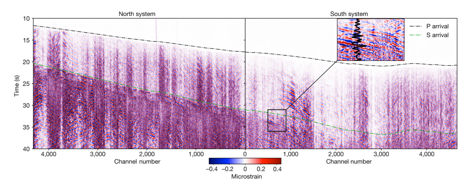
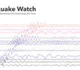
Figure 3: Record of Mw 6.0 event approx. 150 km from the interrogator location. Two DAS cables run from two separate interrogators (location of interrogators at Channel number 0) hosted in the town of Old Mammoth, California, United States. The DAS cables are each 50 km long and sampled at 200Hz. In the figure you can see clear arrivals of the P- and S-waves. Adjusted from Li et al., (2023).
An amazingly detailed picture of the wavefield, without having to deploy geophones! Next up is an earthquake in Mexico which is far away from the recording interrogator in Stanford.
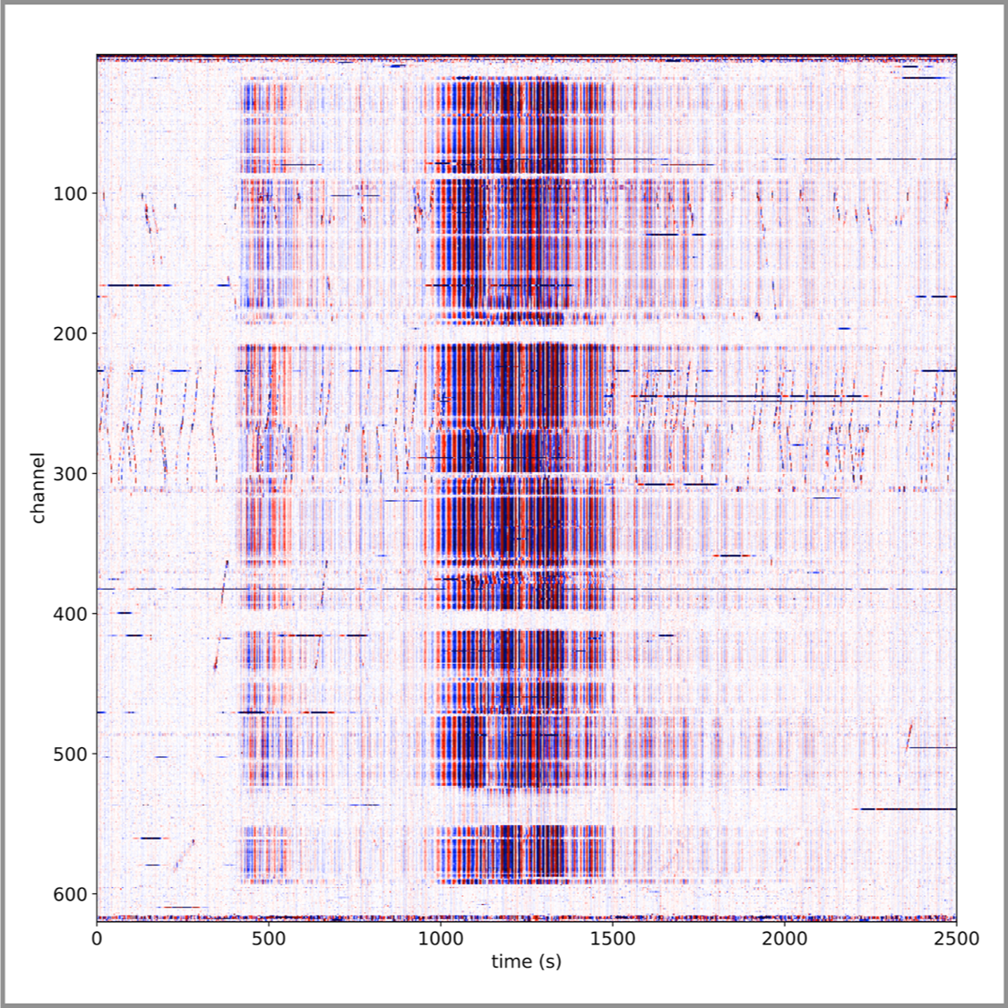
Figure 4: Record at seismic fiber optic observatory of Stanford university from an 8.2 magnitude earthquake occurring in central Mexico on Sept. 8, 2017. Also here a clear P- and S-wave arrival are visible. Worth noting is the lack of move-out visible between the channels. This is due to the cable configuration (a 3 mile figure eight) and the large distance between the cable and the epicenter ( more than 2000 km). (Image credit: Siyuan Yuan, obtained from: here)
Borehole DAS data:
When fiber-optic cable is cemented outside of the casing of a borehole, it is well coupled to the bedrock, and the borehole can still be used for other things in the meantime! This is a great advantage of DAS, because downhole geophones can be costly, are probably less densely spaced, have temperature limitations, and they block the borehole! However, their 3-component data is still relatively indispensable, where DAS in a straight borehole is only 1-component. Take a look at the amazing data of borehole DAS for monitoring microseismicity during a stimulation (2022) in the Utah FORGE geothermal test site:
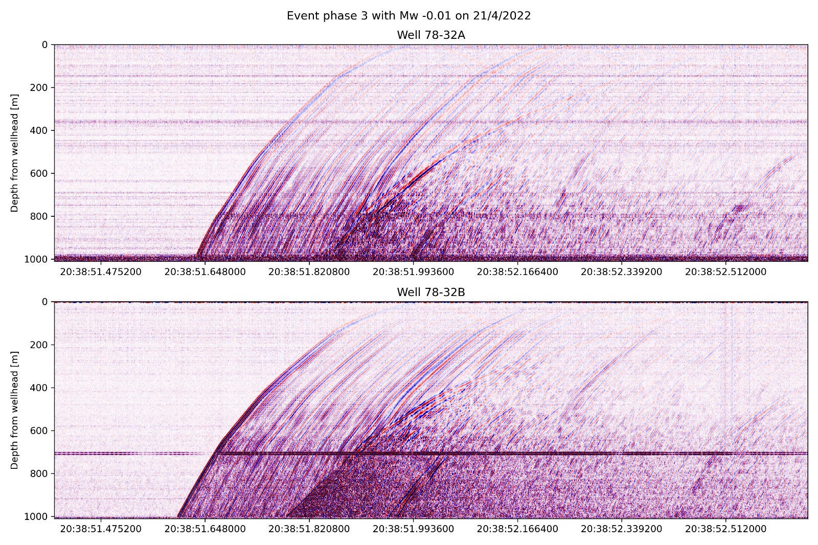
Figure 5: Image from a microseismic event coming from below on 2 boreholes (Utah FORGE, April 2022 stimulation dataset (Data in GDR repository, see Martin and Nash, 2019, image by Katinka Tuinstra).
Glacier DAS data
Fiber-optic cables are also great candidates for glacier seismology. They can couple to the ice by melting into it! Examples are studies from Greenland (Fichtner et al., 2023) and Antarctica (Hudson et al., 2021), or take a look at the data from the Rhône Glacier in Switzerland:
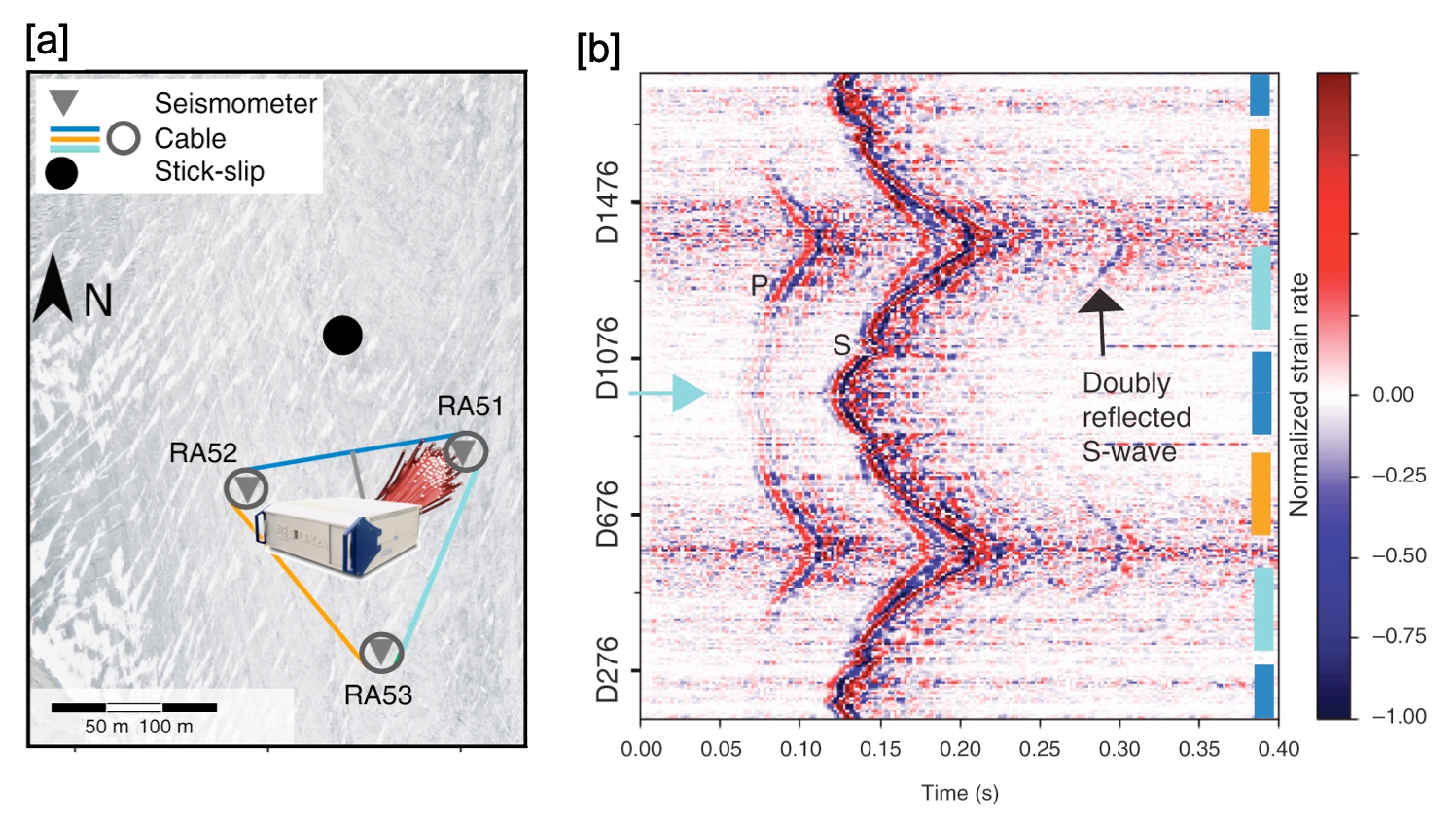
Figure 6: DAS data from a glacier setting. [a] the triangle DAS cable layout on Rhone Glacier, Switzerland, where the colors of the cable correspond to the cable segments as depicted in [b]. The black dot corresponds to the event shown in [b]. [b] Full DAS record of stick-slip event, with on the y-axis the channel numbers. The clearly visible symmetric move-out is caused by the triangle configuration of the DAS cable. Clear P- and S-wave arrivals can be seen and even some doubly reflected S-waves. (Adapted from Walter et al. (2020)).
Exciting applications of DAS
Fiber-optic cable is everywhere. That’s why it can also be used for many exciting and out-of-the-box applications. Recently, the ETH Zürich, in collaboration with Icelandic Met office IMO and HS Orca, started monitoring the seismic sequence and potential eruption in Grindavik, Iceland. They set up a livestream (click here) for everyone to watch, have a look! Another exciting application is whale tracking, where subsea cables have been used to locate and track different whales by their songs that were recorded with DAS (Rørstadbotnen et al., 2023). Of course, fiber-optic cables can also be deployed inside boreholes (cemented outside of the casing, for example). Recently, the DAS community came together in the DAS month (Wuestevelt & Spica et al., 2023) and recorded at the same time with many instruments in February 2023. Many instruments recorded the destructive Mw 7.8 and 7.7 Turkey earthquakes on the 6th of February (as presented on EGU by Jousset et al., 2023).
Get started with community datasets!
We’ve only lifted the tip of the iceberg for you now. There are also other fiber-optic sensing techniques, including DSS (Distributed Strain Sensing), DTS (Distributed Temperature Sensing), and many others! Did we already spark your interest? Try having a look at some DAS data yourself: IRIS/EarthScope offers more information and links to some open-access datasets. Other open access datasets include:
The era of fiber-optic measurements in various disciplines of geoscience has only just started. Just have a look already at the submarine fiber optic cables of the world! Although DAS in it self can not surpass the 200 km range yet, other methods are already there. But who knows where we’ll be in 10 years: stay tuned!
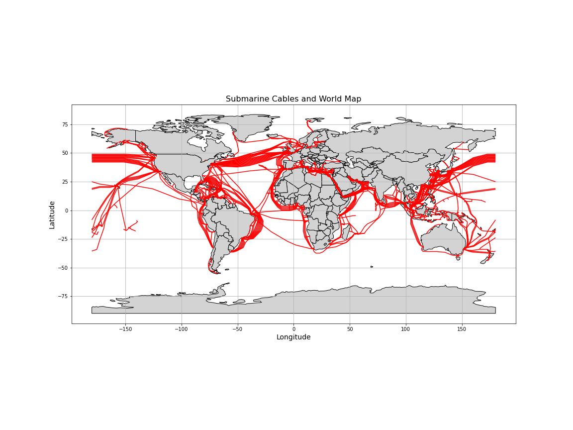
Figure 7: Submarine Cables and Terminals (2018): data taken from here, figure made with the Cartopy library by Katinka Tuinstra.
REFERENCES
Jousset, Philippe, et al. Global Distributed Fibre Optic Sensing recordings of the February 2023 Turkey earthquake sequence. No. EGU23-17618. Copernicus Meetings, 2023.
Nap, Ana, (2020), On the fidelity of Distributed Acoustic Sensing (Master thesis), ETH Zürich, Switzerland.
Dedi Purwana
It’s an interesting article!
Sharon Jones Davis
WOW! Interesting I use Strain rate to interrogate the heart! Cardiac Sonographer since 1989!
Mawarslot
thanks for the great article treat
Daniel Pyke
There is a nice video explanation / animation of how Distributed Acoustic Sensing works here – https://www.sensonic.com/en/blog/what-is-distributed-acoustic-sensing-how-does-it-work–3274/ for those that prefer to learn more visually.