Seismic Denoising meets Generative Image Models

'Santa Claus Looking at a Seismic Trace on a Monitor' created by DALL-E 3

What’s the connection between novel generative image models and seismic denoising? Daniele Trappolini from Sapienza Università di Roma has led an effort to utilise these exciting techniques for seismological applications. This blog post will give a beginner-friendly introduction to generative modelling and ‘diffusion’ models, before explaining how Daniele and his group have been using them to push the limits of seismic denoising. Buckle up!

Generative Image Models

Generative image models have surged to prominence in the last 18 months, with a spate of advances leading to many highly popular applications. Perhaps the most important improvement in the field is the introduction of diffusion models, which have revolutionised generative modelling using Machine Learning (ML). These models have proven incredibly powerful in modelling complex distributions of high dimensional data, and have seen particular success in image and audio generation. In part enabled by improvements in ML-based language modelling, a number of diffusion models gained prominence for their success in generating highly detailed and diverse images given text prompts.

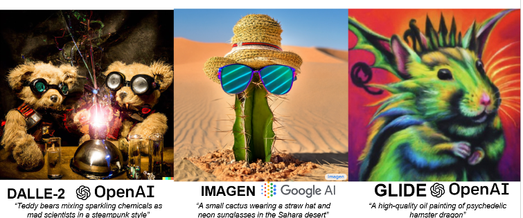
Fig. 1: Examples of images drawn from several popular generative diffusion models. Each model takes a text input as a prompt and generates the associated image. Since these models are probabilistic, the same prompt can yield distinct, diverse images each time.

Generative Modelling

Generative models are trained on a dataset of observations D = {x} to model their distribution p(x), where the dataset could be images of dogs, spectrograms of speech, or even seismic traces. This modelling is performed by particular types of neural networks (such as a Convolution Neural Network), generally chosen for the specific data structure at hand. Once trained, the models can be evaluated to sample from their representation of p(x), producing a newly generated observation x ~ p(x).

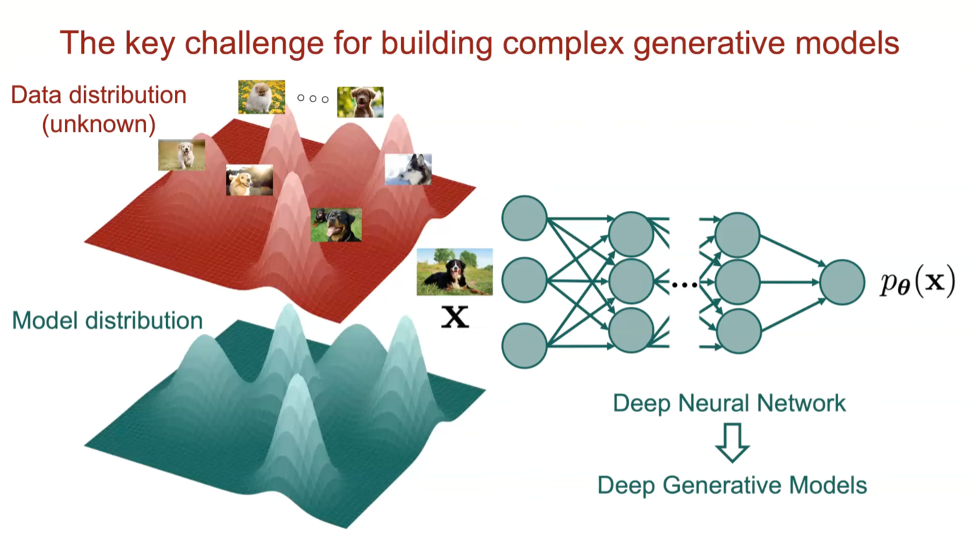
Fig 2: The data distribution of dog images is modelled using a deep neural network, which aims to learn this distribution from lots of examples. The data can be high dimensional and complex, with many different modes (shown as peaks of p(x)). Adapted from a tutorial by Yang Song, Stanford.

Until the advent of diffusion models, there were two key models used in generative modelling: Generative Adversarial Networks (GANs) and Variational Autoencoders (VAEs). These models train a neural network to directly model p(x), such that once trained, a random seed can be fed into the neural network to generate a new sample x ~ p(x). This proved highly effective and efficient – check out thispersondoesnotexist.com and keep refreshing for a neat (or worrying?) example. These models have also been used in seismology, with applications in data augmentation (e.g. Li et al (2018) [1], Wang et al. (2021) [2]) and waveform generation for accelerated inference (e.g. Spurio Mancini et al. (2021) [3].)

GANs and VAEs have their limitations, however; since p(x) may be extremely complex in high dimensions, models often fail to capture the entire distribution. Modelling all of p(x) accurately is a tough task; the models can miss or blur over ‘modes’ (shown as peaks in the distributions above). These skewed distributions may only capture parts of the data distribution, or, worse, leads to generated examples that don’t look right or are completely unrealistic.

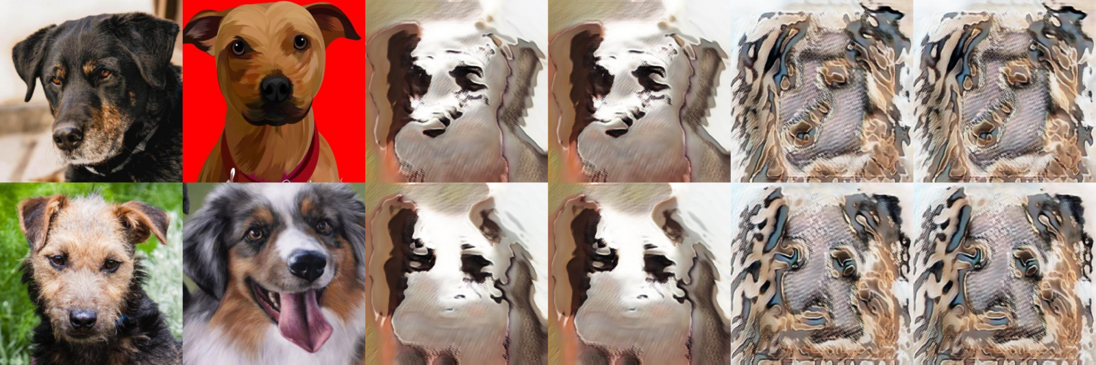
Fig. 3: A typical example of ‘mode collapse’, a common failure mode of GANs and VAEs.

Diffusion Models

Diffusion models represent a paradigm shift in modelling the distribution of the data p(x). Instead of training a neural network to model the whole distribution, the diffusion framework trains a model to learn its gradient ∇p(x). The model can then be repeatedly evaluated to perform a type of gradient ascent, aiming to find one of the many peaks of the data distribution p(x). This novel approach, in conjunction with several practical and theoretical advances, allows diffusion models to produce highly detailed and diverse samples, since it can consistently draw samples from the very peaks of the data distribution p(x).

Fig. 4: A noisy gradient ascent algorithm that utilises the gradient ∇p(x) to draw samples from the peaks x ~ p(x). The arrows show the gradient ∇p(x), and each blue dot performs the gradient ascent toward the peaks of p(x). For the technically minded, there is close connection between diffusion model sampling and Langevin Monte Carlo (LMC), generally used to draw samples from high-dimensional distributions where simpler sampling techniques like Metropolis-Hastings are insufficient. Adapted from a technical blogpost.

But how do you learn the gradient of a probability distribution using only discrete samples D = {x}? The key idea is to add noise to your data x (hence disturbing it from the distribution p(x)), and then teach a model to remove that noise. By training the model to move from noisy versions of the data towards the real data, it learns to model the gradient ∇p(x).

Denoising Diffusion

So we train a ML model to remove synthetic noise from our data observations. In practice, it is useful to do this over different amounts of noise – the simplest idea is to gradually add Gaussian noise to the image, leading to something resembling… diffusion! The original paper to demonstrate this approach named it Denoising Diffusion Probabilistic Models [4].

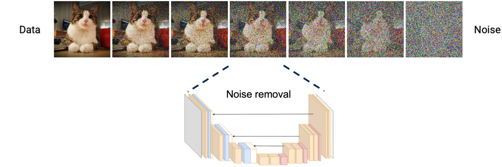
Fig. 5: In diffusion models, synthetic noise is added to an image (left-to-right) and a neural network is trained to remove it (right-to-left). This teaches the neural network model the gradient of the data distribution ∇p(x). Adapted from a comprehensive CVPR2022 tutorial.

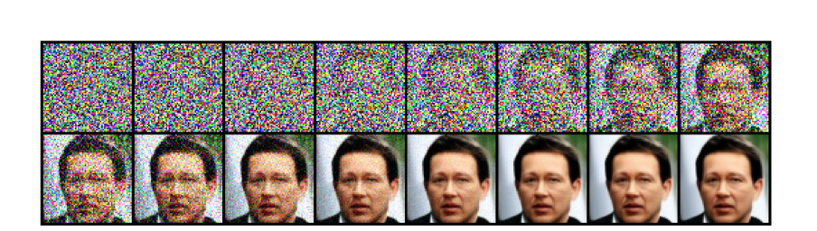
Fig. 6: Once trained, the gradient can be used to perform various types of gradient ascent, allowing us to produce diverse and high quality samples from the data distribution p(x). Figure from Tachibana et al. [5]

This concludes the brief background to diffusion models. They have seen tremendous interest both within and outside of the ML community. Another example of their applications outside of seismology include audio generation, which produce realistic sounding audio by performing diffusion in the time-frequency domain (i.e., images of spectrograms). Some examples include:

Text-to-speech: Guided TTS [6]
Text-to-audio and text-to-music models from Meta [7]

Follow the links for example audio!

CDiffSD: Cold Diffusion for Seismic Denoising

Daniele Trappolini and his group at Sapienza Università di Roma have adapted diffusion models for seismic denoising. In their quest to find a model capable of effectively denoising seismic traces, diffusion models presented an ideal starting point due to their robustness in handling complex data patterns. However, a key challenge in seismic data analysis is the predominantly non-Gaussian nature of noise, which standard diffusion models, relying on Gaussian noise, are not equipped to handle optimally. This led them to the adoption of cold diffusion models, an evolution of the standard diffusion framework. Cold diffusion models are designed to work with a broader spectrum of noise types, including non-Gaussian noise, making them particularly suited for seismic applications where the noise characteristics are complex and varied.

Given the non-Gaussian nature of seismic noise, the simplest diffusion approaches discussed above face limitations. Cold diffusion, on the other hand, generalizes this concept by using non-Gaussian noise, making it more adaptable to the complexities of seismic data. This versatility is crucial, especially in practical settings where noise types can vary significantly. Cold diffusion therefore represents a huge leap forward for applying these novel ML techniques for seismic denoising.

Trappolini et al. [8] introduces the CDiffSD model, a specialized adaptation of the cold diffusion model for seismic denoising. This model stands out for its tailored approach to the unique challenges of seismic data. In the context of diffusion models, two key processes are crucial: the ‘forward process’ and ‘sampling.’

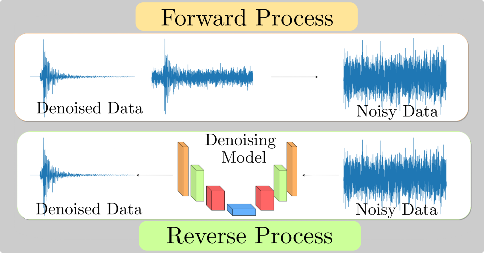
Fig 7: An adapted diffusion framework for seismic data denoising, introduced here as CDiffSD.

Forward Process: In diffusion models, the forward process involves gradually adding noise to the original clean data. For seismic data, this means progressively introducing various types of noise to the clean seismic signals. This process transforms the original signal into a noisier version, mimicking the real-world scenario where seismic data is often contaminated with various forms of noise.

Sampling: The sampling process is the reverse of the forward process. It involves iteratively removing the added noise to recover the original signal from the noisy data. In the case of CDiffSD, this process is enhanced to specifically cater to the complexities of seismic noise, which often deviates from standard Gaussian noise. By refining the sampling algorithm, CDiffSD can more effectively separate the seismic signals from the noise, resulting in cleaner and more accurate seismic data.

The CDiffSD model, with its advanced approach to both the forward and sampling processes, is particularly effective for seismic applications, demonstrating improved performance in denoising and preserving the integrity of seismic signals

Performance Evaluation

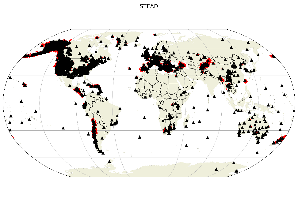
Fig 8: Distribution of earthquakes in the STEAD dataset, image taken from SeisBench (https://seisbench.readthedocs.io/en/stable/pages/benchmark_datasets.html)

This research utilized the comprehensive STanford EArthquake Dataset (STEAD), which was methodically partitioned into training, evaluation, and test subsets. Unlike conventional approaches, a random coupling of noise and earthquakes was ensured, fostering a scalable and robust denoising framework. A notable innovation in the methodology is the channel-specific normalization process, which standardizes seismic data within a specific range, ensuring the relative amplitude characteristics are retained.

In evaluation of the CDiffSD model, the team focused on key metrics like Signal to Noise Ratio (SNR) and cross-correlation, alongside integrating PhaseNet for P and S wave-picking accuracy. This combination offered a comprehensive view of the model’s effectiveness. Notably, the CDiffSD model outperformed traditional denoisers, particularly enhancing PhaseNet’s ability to accurately identify P and S wave arrivals. This improvement highlights the CDiffSD model’s potential in refining seismic data analysis, making it a valuable tool for more precise earthquake characterization.

Fig 9: Trace picked from the test set and denoised with CDiffSD. PhaseNet is then used for phase picking.

Conclusion

The CDiffSD model marks a significant advancement in seismic data analysis. It demonstrates greater adaptability to different types of seismic noise compared to traditional methods. While it shows variability in performance depending on the noise characteristics and signal features, its ability to enhance the fidelity of seismic traces to their original signals is evident. This research opens up new possibilities for more accurate and efficient seismic data analysis. Additionally, it’s worth noting that the same methodology underlying the CDiffSD model could potentially be adapted for generating seismic traces from textual input. This innovative approach would involve interpreting text-based seismic descriptors and converting them into accurate seismic signal representations, further broadening the scope and utility of our model in seismic research and analysis.

We hope you’ve enjoyed this blogpost, which has provided a primer on generative image models and how they have been adapted for seismic data denoising. Feel free to reach out to the authors of this blogpost for comments or questions, or post them down below.

References:

[8] Trappolini, Daniele, et al. “CDiffSD: Cold Diffusion Model for seismic denoising.” AGU23 (2023).