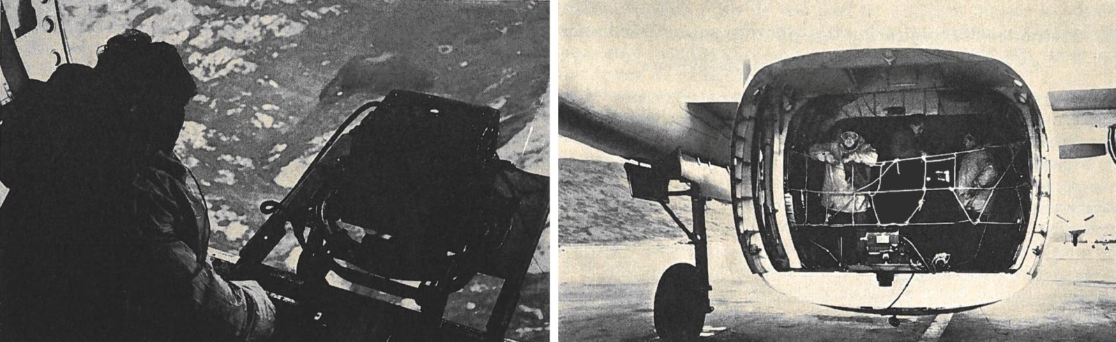
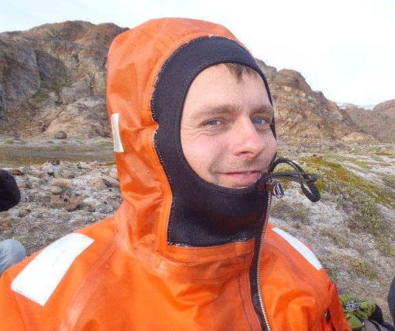
Figure 1. Taking photos from an open, unpressurised aircraft put limitations on flying height, resulting in a small area covered by each photo (2.5 km). A lot of warm clothing was required for the crew. Photos reproduced from Bauer, 1968.
Recent work published in my department at the Geological Survey of Denmark and Greenland (GEUS) focused on solid ice discharge into the ocean from the Greenland Ice Sheet from 1986 to 2017 (Mankoff et al. 2019). Solid ice discharge is the ice that is lost from a glacier as it flows towards the coast and eventually breaks off as icebergs into the ocean (i.e. calving). Solid ice discharge is an important constraint for sea level rise predictions. Today, we use satellite observations and available models. However, during the pre-satellite era, ice discharge had to be evaluated very differently. Read on to learn about what was done during the Expédition Glaciologique Internationale Au Groenland 1957–60 (EGIG), claimed to be the first of its kind (Bauer, 1968).
The EGIG was a joint expedition between Denmark, France, Germany and Switzerland during the International Geophysical Year (1957-58). This expedition saw a lot of fieldwork on the ground, but also calculated solid ice discharge from the ice sheet using aerial photos from airplanes. The photos were collected during surveys in 1957, ‘58, ‘59 and ’64 flown by the French air force and the Danish Geodetic Institute. Repeated flights allowed them to map the surface velocity of 20 glaciers along the west coast of the Greenland Ice Sheet (Fig. 2). By taking repeat photos two weeks apart, it is possible to measure how much the ice has moved in the time interval. In addition, they collected glacier elevation profiles using radar altimeters needed for their calculations.
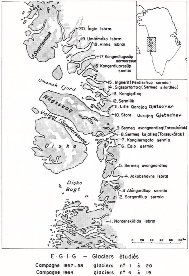
Figure 2. Original map of the glaciers surveyed in 1957/58, 1959 and 1964. Figure is shown unmodified from Carbonnel & Bauer (1968).
Assuming that the ice is perfectly slippery at the base and so flows as a “plug”, three inputs are needed to calculate solid ice discharge: surface speed at the line where the glacier is still ”attached” to the bedrock below, the width of the glacier, and the average ice thickness of the glacier.
Today, we use optical and radar data from satellites to calculate surface speeds by tracking features over time. Finding the thickness of outlet glaciers can still be problematic, as radar signals are often prevented from imaging the bedrock below the glaciers due to the presence of water in the ice. And, until recently, the bathymetry of the fjords into which the glaciers flow was sparse. The OMG project has done a lot to rectify this, by sounding many Greenlandic fjords, and applying a physical model to fill out the gaps in the data sets.
When the EGIG set out in 1957, the first year of photo flights collected by the French air force was intended as a trial run, to determine the best practices and equipment. Due to the use of unpressurised aircrafts, this limited the altitude of flight, resulting in a small area covered by each photo of 2.5 x 2.5 km (also called the ground footprint). This information was passed on to the Danish Geodetic Institute who took over from 1958. The Danish surveys used wide angle mapping cameras and an aircraft with pressurized cabins, allowing for a higher altitude of flight. Their more modern and suitable equipment allowed to photograph a much wider view of the glaciers with a 11 km ground footprint. All glaciers had already been successfully surveyed from the air in 1957 – except for Jakobshavn Isbræ (JI), where the aircraft navigation procedure had failed (see Fig.3). JI was also too large a glacier to survey entirely with the reconnaissance camera used by the French air force. The Danish Geodetic Institute flew over JI in 1958, allowing to make the first map of the surface velocity of JI, and thus completing the 1957/58 aerial survey.

Figure 3. A strip of photos taken in an attempt to photograph Jakobshavn Isbræ in 1957. Two strips of aerial photos taken some time apart are needed to measure how glaciers move. This strip missed Jakobshavn Isbræ, as it mostly captured the water and therefore did not overlap with the second (repeat) strip. This made it unsuited for measuring the Jakobshavn Isbræ’s speed.
The Danish team returned in 1959 with the intention to collect repeat photos along the whole ice sheet margin already surveyed the previous years. They succeeded in repeating the first round of flights, but poor weather conditions prevented them from repeating all the flights within the allotted month. Again, JI remained elusive due to mechanical failure in the camera that caused the loss of two photos over JI. In 1964, the Danish team returned with a vengeance to do repeat flights focusing on the glaciers flowing directly into the ocean only (i.e. marine-terminating) and were finally successful with repeat intervals of 12-13 days between photo repeats.
Today, we use computers and image-correlation techniques to track how a glacier moves in the time interval between the acquisition of two images. The EGIG made their maps of glacier flow by manual image-correlation. For this procedure, you would make a copy of the photo on “Astrafoil”, a (plastic) cut-out of the area you want to measure, and manually move the transparent cut-out until you found a match. This procedure worked best if the photos had been recorded at the same time of day, casting similar shadows in the crevasses. Finally, by reconstructing the coordinates of the start and end point in 3D space, the displacement could be computed (like in Fig.4).
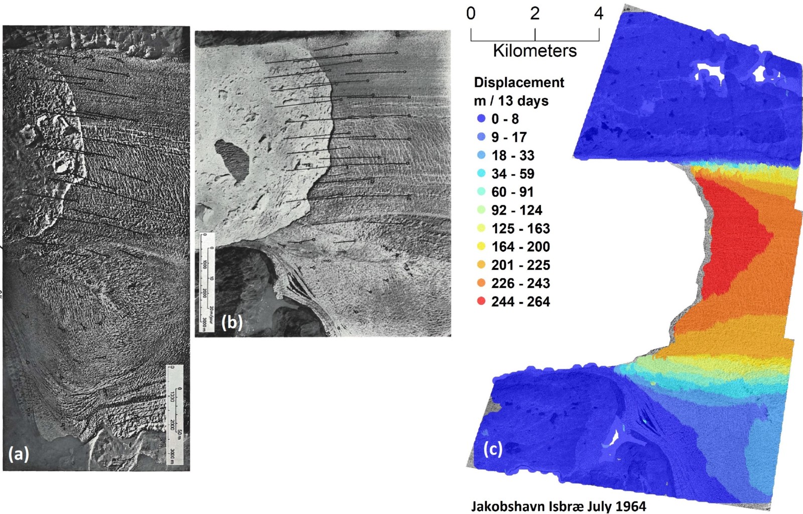
Figure 4. (a) shows the earliest velocity map of Jakobshavn Isbræ from the year 1958, (b) shows the velocity map of Jakobshavn Isbræ from 1964. They were both measured manually. Both images are unmodified from Bauer (1968) and Carbonnel and Bauer (1968). (c) is the 1964 velocity map but this time digitally processed using image correlation.
Where did EGIG get data on ice thickness? They could measure the height of the ice by using the photographs and radar altimeters onboard the aircraft. Since the glaciers they were surveying were marine-terminating, the height of the glacier represented the ice thickness above water. The remaining ice thickness below the water surface would have had to be estimated using existing depth soundings of the fjords. Because only half of the fjords had data available, the depths of the other half were then estimated by looking at aerial photos of newly calved icebergs lying sideways and assuming that the glacier filled the whole fjord cavity. The height of the glacier front measured from the photographs could also be used to obtain the depth of the fjord below sea level at the grounding line by subtracting it from the iceberg height.
With known surface speeds, glacier thickness and glacier width, EGIG was able to calculate the solid ice discharge of the marine-terminating glaciers of the Greenland Ice Sheet terminating in Disko Bugt and Uummannaq Fjord as early as 1957/58!
Further reading:
- Andersen, E., 1968. Report of the Geodetic, Geophysic, and Photogrammetric Work at the West Coast Region of Greenland: Executed by the Danish Geodetic Institute in Connection with the Ice-cap Work of EGIG. CA Reitzels Forlag. Monographs on Greenland, 173, 4.
- Bauer, A., 1968. Missions aeriennes de reconnaissance au Groenland 1957-1958; observations aeriennes et terrestres, exploitation des photographies aeriennes, determination des vitesses des glaciers velant dans Disko Bugt et Umanak Fjord. Monographs on Greenland, 173, 3.
- Carbonnel, M. and Bauer, A. 1968. Exploitation des couvertures photographiques aériennes répétées du front des glaciers vêlant dans Disko Bugt et Umanak Fjord, Juin-Juillet 1964. Monographs on Greenland, 173, 5.
- Mankoff, K.D., Colgan, W., Solgaard, A., Karlsson, N.B., Ahlstrom, A.P. van As, D., Box, J.E., Khan, S.A. Kjeldsen, K.K., Mouginot, J. and Fausto, R.S. 2019. Greenland Ice Sheet solid ice discharge from 1986 through 2017, Earth System Science Data, 11, 2 769-786, doi:105194/essd-11-769-2019.
- Link to Department of Glaciology and Climate at GEUS.
Edited by Marie Cavitte
 Niels J. Korsgaard is working as a glaciologist in the Department of Glaciology and Climate at the Geological Survey of Denmark and Greenland (GEUS). He has a MSc in Geography and Geoinformatics and a PhD in Geology and Geoscience. His main focus is remote sensing of the Greenland Ice Sheet and its peripheral glaciers, with a decade-old interest in historical aerial photos of Greenland. Contact email: njk@geus.dk. He tweets as @NielsKorsgaard
 Baptiste Vandecrux obtained a M.Sc. in engineering science both from Ecole Centrale de Lille (France) and from the Technical University of Denmark (DTU) in 2015. From 2015 to 2019, he conducted a PhD co-hosted by DTU and the Geological Survey of Denmark and Greenland (GEUS). His thesis focused on firn meltwater retention processes on the Greenland Ice Sheet, using firn cores, weather station data and firn models. He is now a postdoc at GEUS and works on optical remote sensing of snow and firn modelling in the department of Glaciology and Climate. Contact email: bav@geus.dk