Ice cores are a favored archive to study past climates, because they provide a number of indications on the history of the climate and of the atmospheric composition. Among these, water stable isotopes are considered as a very reliable temperature proxy. Yet, their interpretation is sometimes more complicated than a simple one-to-one correspondence with local temperature and requires intercomparison with other proxy records, as various processes affect the signal found in the ice cores.
How does it work?
All water molecules are not equal: some are heavier due to one of their atoms being substituted with a heavier counterpart (the standard oxygen molecule, 16O, can be substituted by an 17O or an 18O, whereas the hydrogen (H) can be substituted by a deuterium (D=2H)). These molecules (e.g. H216O, H218O and HD16O) are called isotopologues (or isotopes in short, but it’s technically inaccurate), and have each different physical properties. As a result, the molecules react differently to external factors, leading to fractionation (processes that affect the relative abundance of isotopes). The isotopic composition (commonly referred to as δ18O, δ17O and δD) of snow is governed by fractionation from the evaporation site, where the moisture first enters the atmosphere, to the precipitation site where it is deposited to the ground (Dansgaard 1953)(see video below). First, over the ocean, the heavier isotopes are less likely to take part in the formation of moisture, leading to lower concentrations of the heavy isotopes in the clouds compared to the mean oceanic water isotopic composition (lower concentration means that the δ18O is more negative). Then, as the air masses move toward the poles, temperature decreases leading to precipitation (either liquid or solid). The heavier isotopes will be preferentially found in the condensed phase than the light ones, which depletes even more the cloud from its heavy isotopes. Finally, in remote areas of the Polar Regions, the isotopic content of the final precipitation results from successive precipitation events. Since, as we saw, the precipitation contents in each isotope are different, each successive precipitation event will have a different isotopic composition, with the final one having the least heavy isotopes – a process called distillation. At each step of the moisture’s path from ocean to cloud to precipitation, the isotopic fractionation is strongly influenced by temperature. This leads to a temperature signal in the isotopic composition of both vapour and precipitation.
This video shows the isotopic fractionation at each step of the water cycle (from the evaporation over the ocean to the location where the precipitation occurs) are integrated, giving the temperature and humidity sensitivity of the isotopic content of the precipitation (modified from Casado (2016)).
Over glaciers and ice sheets, snow accumulates and can remain preserved for hundred of thousands of years. Thus, analysing the isotopic composition of these successive layers enables us to retrieve past temperatures. Considering the very low amount of water necessary to obtain a measurement, analysing an ice core can provide continuous and high-resolution time series of past climatic variations.
A classic way to retrieve temperature from isotopic composition data is to use the spatial relationship between δ18O of surface snow and surface temperature (e.g. Lorius and Merlivat (1975) for Antarctica). That is, to measure simultaneously the present-day temperature and the δ18O of surface snow across the study area and to make use of their linear spatial relationship to infer past temperatures from the δ18O of the ice core. However, one should keep in mind two main limitations when using such a method. First, it assumes that the spatial relationship between δ18O and temperature is a good surrogate for the temporal δ18O versus temperature relationship. However, this link is known to change with time (and hence depth of the snow deposit). Second, processes occurring after the snow has fallen, such as sublimation or blowing wind, can affect the way the snow is layered in the ice core, as well as its isotopic composition.
Resolution and noise
The local accumulation (expressed in cm of snow per year) is a determining factor for both the extent of an ice core record and the maximal resolution that can be achieved. As the present-day ice thickness is capped between 3 and 4 km, it is necessary to choose a site with low accumulation to obtain an ice record spanning several glacial/interglacial (i.e. warmer and colder) cycles (Fischer et al. 2013). For instance, the NGRIP ice core in Greenland was retrieved in one of the thickest part of the Greenland ice sheet (see Figure 1. b)). Similarly, the Dome C ice core (the ice core spanning the furthest in the past to date which is 800,000 years before present) was retrieved in an area of Antarctica where the ice sheet was very thick (more than 3000 meters) and the accumulation very low (roughly 2.5 cm per year).
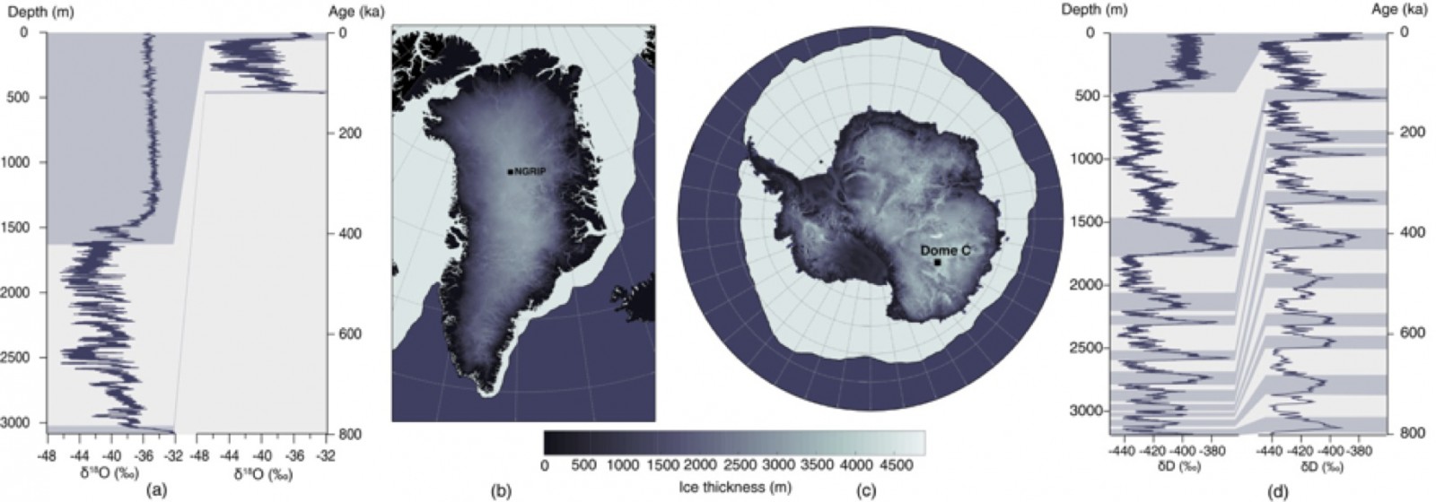
Figure 1: Greenland and Antarctic ice core sites: (a) Isotopic signal from the NGRIP, (b) and (c) maps of ice thickness in Greenland and Antarctica, respectively, and (d), isotopic signal from the Dome C. The isotopic signal for both sites is presented against the depth (left) and with the associated age model (right), warm periods are shown in grey to indicate the correspondence between age and depth in the ice cores (Casado et al, 2017).
For sites with low accumulation, the snow stays exposed at the surface for a long time. Hence, the initial precipitation signal is modified by local processes occurring after the snow has fallen (Ekaykin et al. 2002). This prevents proper recording of the signal at timescales below several years, for sites with accumulation lower than 8 cm per year (Münch et al. 2016). Deeper in the ice, diffusion processes smoothen the isotopic composition time series, erasing part of the climatic signal (Johnsen 1977). This limits the interpretation of ice core records at time scales smaller than a few decades. Finally, retrieving a temperature signal at high resolution for longer time scales remains a challenge because of the varying relationship between δ18O and the temperature deeper in the ice. The first limitation is the accumulation rate itself, which is typically lower during glacial periods. The temporal resolution also gets lower with depth as the ice thins due to the increasing pressure exert by the overlying ice layers. As illustrated in Fig. 1, the number of years per meter globally increases with the depth of the record, from roughly 20 years per meter at the top of the core at Dome C up to 1,400 years per meter for glacial periods at the bottom. Overall, the variability found in single ice core records combines both the climate variability and several signatures from other local processes affecting the snow.
Isotope-temperature calibration
The temperature signal retrieved from δ18O can be tested against independent temperature time series, such as borehole temperature measurements at the ice core site, to aid in reconstructing the correct δ18O versus temperature relationship (the so–called “calibration” process). The temperature of the borehole from which the ice core was extracted is measured at different depths. Small variations in these temperatures provide a reliable but low-resolution measurement of past temperature changes as the ice is a good thermal insulator. Measurements performed in Greenland have suggested that the use of the spatial δ18O versus temperature relationship described above underestimates by a factor of two the magnitude of the temperature change between the last glacial maximum (LGM, the last period when ice sheets were at their peak extension) and the present-day (Cuffey et al. 1994). Jouzel et al. (2003) confirmed this using computer simulations, and further showed that the δ18O versus temperature relationship does not remain constant over time. This large variability can be due to differences in the large-scale atmospheric circulation, vertical structure of the atmosphere, seasonality of precipitation, modification of location of the moisture source regions or of their climatic conditions.
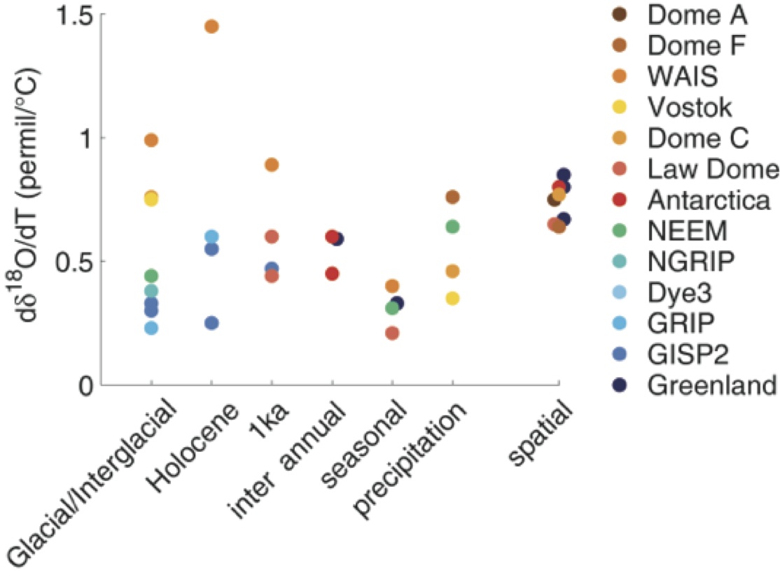
Figure 2: Relationships between isotopes and temperature for different locations and timescales (indicated along the horizontal axis). A higher value would lead to higher temperature difference estimate for the same δ18O difference (Casado et al, 2017).
Calibration of the isotopic paleothermometer is therefore essential, and is realised through different methods. Station data can be used at the seasonal and interannual scales, isotopes of other gases at decadal to centennial scales (Guillevic et al. 2013) and borehole temperature measurements at millennial scales (Orsi et al. 2017). Finally, climate models which represent isotopic processes (called “isotope-enabled”) can be used to infer the isotope-temperature relationship with a direct control on the time scale and on the period. For instance, Sime et al. (2009) highlighted that for warm interglacial conditions, the isotope-temperature relationship can become non-linear whereas it is not the case for cooler (glacial) conditions.
The δ18O versus temperature relationships found in the literature (Fig. 2) span values ranging between 0.2 ‰/°C to 1.5 ‰/°C. From this compilation, it is clear that a more complex framework than simple linear regression to temperature is necessary to interpret the isotopic signal.
Conclusions
If water isotopes from ice core records are insightful tools to reconstruct past climates, there are fundamental limits to their power of reconstruction.
The above therefore calls for a careful use of isotopic records when these time-series are used for general inferences about the climate system (e.g. Huybers and Curry (2006)). A possible way forward is to use isotope-enabled global climate models (Sime et al. 2009). A complementary approach is to undertake process field studies (Casado et al. 2016), which can help to evaluate how the isotopic signal is modified after the deposition, and how the relationship between isotopes and temperature is altered at the seasonal and inter annual timescales.
The Beyond EPICA – Oldest Ice project plans to retrieve an ice core in Antarctica in which over 1.5 million years of climatic record could be retrieved. This will enable to go further back than the 800, 000 years old ice core obtained at Dome C and thus, would be a breakthrough into studying the changes in orbital forcing during the mid-Pleistocene transition (900 to 1,200 thousand years ago) during which the glacial-interglacial cycles shifted from lasting 41, 000 years on average to 100, 000 years.