In 1904, the Swedish chemist Svante Arrhenius suggested that the burning of fossil fuels to satiate our hunger for energy would increase the percentage of carbon dioxide (CO2) in the atmosphere, which would change the Earth’s temperature. Regular measurements of atmospheric CO2, started in the late 1950’s at remote locations such as Mauna Loa in Hawaii and the South Pole, confirmed his hypothesis about increasing CO2, with one important caveat. The rate at which CO2 was accumulating in the atmosphere did not match the rate at which it was being produced by fossil fuel burning. In fact, the atmosphere was apparently retaining only half of what was pouring in. Figure 1 shows the observed atmospheric mole fraction of CO2 – moles of CO2 per mole of dry air, usually expressed in “parts per million” – changing with time, along with the change we would have expected if all our fossil fuel emissions would have stayed in the atmosphere.
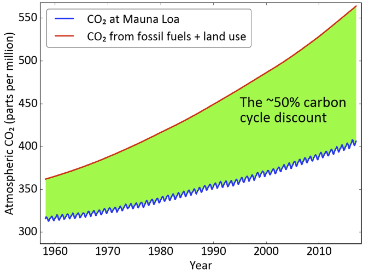
Figure 1: Measured (CO2) mole fraction (moles of (CO2) per mole of dry air) at Mauna Loa, Hawaii in blue, which is a good approximation to the global average atmospheric (CO2). In red is what the global average mole fraction would have been if all the fossil fuel and land use change (mostly biomass burning) emissions since preindustrial times had accumulated in the atmosphere. The green shaded area, therefore, is (CO2) that was emitted due to human activity but did not stay in the atmosphere. Compared to the preindustrial baseline of 280 parts per million (ppm), the (CO2) accumulated in the atmosphere is roughly half of what was emitted. Monthly mean Mauna Loa (CO2) measurements from the Scripps Institute of Oceanography (SIO, http://scrippsco2.ucsd.edu/) and National Oceanic and Atmospheric Administration (NOAA, https://www.esrl.noaa.gov/gmd/ccgg/trends/), fossil fuel emissions from the Carbon Dioxide Information Analysis Center (CDIAC, http://cdiac.ornl.gov/), and land use change emissions from the Global Carbon Project.
Today, we know that the other half – the fossil fuel CO2 emission “missing” from the atmosphere – is taken up by the land biosphere and oceans. The land biosphere accumulates carbon from the atmosphere by increasing plant mass, while the oceans dissolve atmospheric CO2 as the accumulating fossil fuel CO2 in the atmosphere drives the ocean-atmosphere carbon equilibrium out of balance. Beyond this large-scale picture, however, much still remains uncertain. Which part of the land biosphere – the tropics, the temperate latitudes, or the boreal forests and grasslands – takes up the most carbon? How does that uptake change from, say, a drought year to a rainy year? Do old growth forests and young forests take up carbon differently? To what extent do the land and ocean uptakes respond to natural climate cycles such as El Niño or the Pacific Decadal Oscillation?
Answering these questions accurately will not only tell us how the carbon cycle works today, but also how it might respond to a changing climate in the future. Almost all climate models used today to predict future climate contain a model to simulate the response of the carbon cycle (such as the land uptake of CO2) to future climate forcings such as droughts, floods, and elevated temperatures. The prediction skill of a climate model depends crucially on the fidelity of these carbon cycle responses built into the model. However, for the future land carbon uptake these models do not even agree on the sign of the response. Natural climate variations such as the El Niño Southern Oscillations (ENSO) provide us with experiments to evaluate and improve our understanding of these carbon cycle responses.
ENSO is a climate pattern that involves periodic oscillation in winds and sea surface temperatures over the tropical eastern Pacific Ocean. It represents a major control on the year-to-year variation in temperature and precipitation in the Tropics, going through its El Niño and La Niña phases in an irregular fashion that is still difficult to predict but repeating in roughly four-year cycles on average. Less known is the control of ENSO on the atmospheric chemical composition. The global abundance of several gases including greenhouse gases of the natural atmosphere, such as CO2 and CH4, show a clear relation with ENSO. In the case of CO2, both the land and the ocean contribute to this variation in ways that are not well quantified yet, making ENSO an excellent test for models. Closest to the imagination are probably pictures with vague contours of Indonesian farmland covered in thick smoke during El Nino. Indeed, fire is an important mechanism connecting precipitation variability to CO2 variability.
Figure 2 shows the carbon cycle response to the ENSO cycle, as manifest in the atmospheric mole fraction of CO2. Atmospheric CO2 (as well as other greenhouse gases such as CH4) is measured cooperatively by multiple laboratories at a global network of sampling sites, an effort that began more than fifty years ago with Mauna Loa and South Pole. Our knowledge of the carbon cycle response to ENSO – such as the amount of additional carbon in the atmosphere during a strong El Niño, or the partitioning of that signal into contributing factors such as fires in Tropical Asia versus drought in Amazonia – derives to a large degree from these measurements.
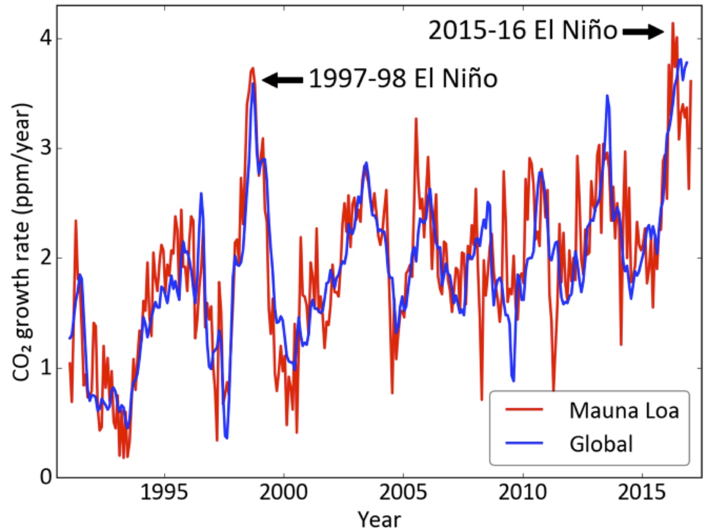
Figure 2: The (CO2) growth rate as measured by the increment of one month over the same month in the previous year. The inter-annual variations in the (CO2) growth rate show a clear imprint of ENSO. Large El Niño events such as the 1997-98 and 2015-16 ones show up as anomalously large spikes in the growth rate. Most of the additional (CO2) in the atmosphere during and after an El Niño comes from the Tropics, and therefore the response measured at Mauna Loa (red) is usually larger than the global average response across a network of background sites (blue). (CO2) data taken from the NOAA (CO2) trends page at https://www.esrl.noaa.gov/gmd/ccgg/trends/.
The atmospheric growth rate of the CO2 mole fraction spikes right after a big El Niño event, such as after 1997-98 and 2015-2016 in Figure 2. Since we know the total mass of air in the atmosphere, we can translate between CO2 mole fraction spikes of Figure 2 and mass of carbon added to the atmosphere. The 1997-98 El Niño added ~2 Petagrams carbon (PgC) to the atmosphere, while preliminary estimates suggest that the more recent 2015-16 event injected ~3 PgC (for comparison, our current global fossil fuel emission is ~10 PgC/year). Having a global network of sites – instead of just background sites such as Mauna Loa – allows us to drill down into the mechanisms behind each of these CO2 increments. For example, we know now that most of the additional 2 PgC carbon from the 1997-98 El Niño was injected from extended fires in the Tropics. Due to the sheer magnitude of the carbon cycle response to El Nino, with the year 2015 setting the record in global CO2 growth to just above 3 ppm/yr, ENSO events present natural experiments against which we can verify our understanding of the interaction between climate and the carbon cycle.
Even for the large changes in CO2 as observed during strong El Nino’s the attribution to specific processes remains a challenge, because of the various coupled responses in the Earth system. For example, the ocean-atmosphere exchange of CO2 is also influenced by ENSO, as shifting patterns in tropical sea surface temperature change the mixing rate of deep and surface waters, influencing gas exchange. Therefore, to get the process-attribution correct, scientist try to disentangle the various influences on atmospheric CO2, which requires a lot of measurements.
Over the past couple of decades, it has become clear that our cooperative network of atmospheric measurements has large gaps over areas that play very important roles in determining the climate impact on the carbon cycle. The gaps are usually due to logistical reasons, such as the difficulty of maintaining measurement sites in Tropical forests, or the expense of making regular shipboard measurements to cover the oceans. To fill this data gap, space based measurements have emerged as a promising yet challenging alternative.
Carbon cycle gases such as CO2 and CH4 (and to a lesser extent CO), by virtue of being greenhouse gases, absorb and emit electromagnetic radiation at certain specific frequencies, usually in the infrared (IR). In theory, a downward-looking IR sensor at the top of the atmosphere should be able to estimate the amount of these gases by measuring the strength of IR radiation at those frequencies. Figure 3 shows the average CO2 mole fraction between the surface and the top of the atmosphere (“column average CO2”) retrieved from the Orbiting Carbon Observatory 2 (OCO2) satellite over Equatorial Africa, showing elevated values due to biomass burning.
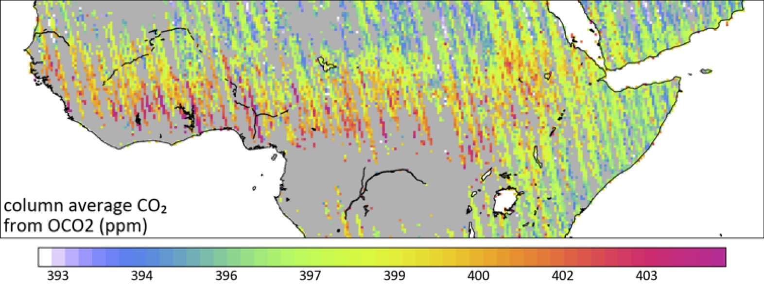
Figure 3: Column average CO2 over Central Africa in 2015 from the Orbiting Carbon Observatory 2 (OCO2) satellite. The bright red band over Equatorial Africa due to biomass burning is visible in contrast to lower (CO2) elsewhere. Column average CO2 from the ACOS algorithm available at https://co2.jpl.nasa.gov/#mission=OCO-2
In practice, IR measured from space is sensitive to many interfering species other than CO2 or CH4, such as the amount of water vapor and dust particles, complicating the estimation of CO2 and CH4 from space. If these complications can be resolved in the near future, space-based measurements could potentially fill the data gap between surface measurement sites (such as Equatorial Africa, which has almost no surface measurements) and enrich our knowledge of the carbon cycle. With such improvements to our measurement capabilities, we hope to better understand today’s carbon cycle and its response to climate. The clearer we see this carbon-climate tango, the better we will be able to predict its imprint on tomorrow’s climate. The most recent climax was one of the most well observed in history. Data are pouring in from multiple sources, and the coming few years promises a lot of interesting analysis as we try to decipher the steps of this complicated dance. Keep your eyes peeled for updates on this blog!
This post has been written by:
Dr Sourish Basu, NOAA Earth System Research Laboratory, USA
Dr Sander Houweling, SRON Netherlands Institute for Space Research, NL
and edited by the new editor of this blog Célia Julia Sapart, Université Libre de Bruxelles, B.