EGU Blogs

Matt Herod

Matt Herod is a Ph.D Candidate in the Department of Earth Sciences at the University of Ottawa in Ontario, Canada. His research focuses on the geochemistry of iodine and the radioactive isotope iodine-129. His work involves characterizing the cycle and sources of 129I in the Canadian Arctic and applying this to long term radioactive waste disposal and the effect of Fukushima fallout. His project includes field work and lab work at the André E. Lalonde 3MV AMS Laboratory. Matt blogs about any topic in geology that interests him, and attempts to make these topics understandable to everyone. Tweets as @GeoHerod.

Some 2014 Ph.D Goal Setting

For my first post of the new year I thought it might be a good idea to make some resolutions, especially since everyone else is doing it. Part of doing graduate work is setting goals, ignoring those goals until the week before, and then working 22 hour days to achieve them. Ian, (my supervisor), if you’re reading this I swear that is just a joke!

Source –  “Piled Higher and Deeper” by Jorge Cham. www.phdcomics.com

In all seriousness though I am hoping that 2014 will be a big year for me. My ultimate goal is to have hopefully defended by this time next year or at the very least submitted my thesis. Of course, I am falling into the obvious trap pictured below by publicly announcing my intent to finish within a year.

Source – “Piled Higher and Deeper” by Jorge Cham. www.phdcomics.com

However, I think that if I set reasonable goals and work really damn hard I can get this thesis done. Hopefully, no major issues occur in the lab or elsewhere that delay things. The easiest way to accomplish this Herculean task is to break it down into somewhat more bite-sized chunks and tackle those one at a time. Trying to think of this as a whole will not help me accomplish anything. Luckily for me uOttawa accepts thesis’s? theses? that are composed of a collection of separate articles, which is the format that I’ll be using.

2014 Goals

– Finish paper on combustion technique – this is nearly done, just have to respond to the journal reviewer comments.

– Continue writing Fukushima paper. Getting there…..this one is not writing itself at the moment, but I am making slow progress every day. If you were at Goldschmidt 2013 you heard this talk.

– Finish all lab work related to iodine and 129I transfer in the Wolf Creek watershed and synthesize data – this is also nearly done, just a few more samples to run on the AMS. Of course the data synthesis and some statistical analysis will take some time.

– Write paper on Wolf creek watershed, make figures, etc.

– Data synthesis and writing of large scale Yukon watersheds project. Got a paper to write here now that I have all the data. Of course there is lots of work to do still on figure making and data analysis as well.

– Learn about noble gas extraction and fissionogenic xenon isotopes…also learn more about stats.

– Start combustion extractions of iodine in Bruce deep geologic repository site core and analyze on AMS and ICP-MS.

– Go to England and analyze xenon isotopes in Lancaster???? Not sure if this is happening yet. Fingers crossed!

–  Synthesise data and write paper on fissionogenic isotopes in ancient groundwater.

– Go to a conference, be it AMS13 in France, GSA in Vancouver, etc….or maybe go to two.

– Get some writing done at the cottage this summer!!!! Very important.

– Staple all this crap together and turn it in.

– Defend! Oh god, I hope this one happens in 2014!

I am flip-flopping between the last two panels at the moment! (Source) – “Piled Higher and Deeper” by Jorge Cham. www.phdcomics.com

Wish me luck, oh yeah, I have to do some blogging here and there as well. On that vein, I would love to have a few more guest posts, since as you can see I am going to be busy this coming year. So if you read this, and are interested in sharing your research, please contact me in the comments or on twitter and we can arrange something.

Matt

Guest Post: Hilary Dugan – Ice as a platform for understanding lake ecosystems

Guest Post: Hilary Dugan – Ice as a platform for understanding lake ecosystems

Today we have a new guest post written by current PhD candidate and Antarctic researcher on her very fascinating field work. Actually, she wrote this post while at McMurdo station. Hilary and I have known each other since our time at Queens University in Kingston, when she was one of my TA’s and was doing her masters. For more info about her work see the bio at the end of the post at check out her own excellent blog.

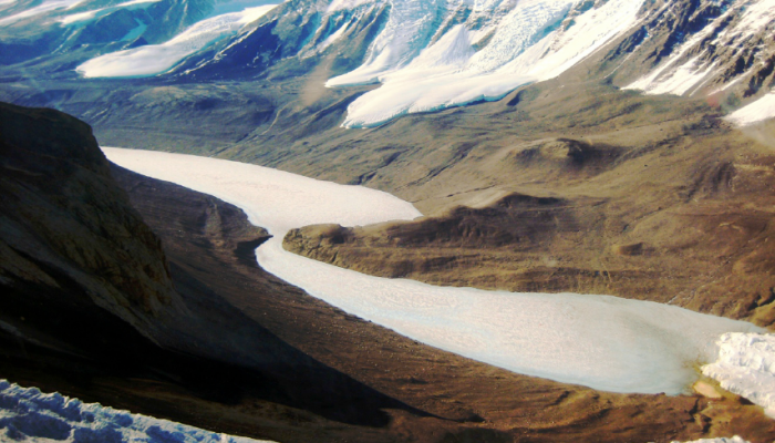
In Antarctica, there is a small swath of land hidden by the Transantarctic Mountains that is too dry and sheltered to be overridden by the ice sheets that cover over 99% of the continent. In these barren valleys, life is at the edge of existence and sustained by pulses of meltwater that form when summer temperatures finally break the freezing point. The only refuges of perennial water in this habitat are the large lakes that occupy the topographic depressions in the valley bottoms. The lakes themselves are hidden beneath permanent ice covers of 4 m, but reach depths of 20 to 75 m, and temperatures of -13 degC to +25 degC. As a colleague remarked, “This system of valleys is one of the coldest and driest places in the world and has more in common with Mars than it does with your backyard”.

1

Don Jon Pond (the saltiest body of water on Earth) in Wright Valley, Antarctica

The McMurdo Dry Valleys is also one of the only places in the world with year-round lake ice, which is partly why I spend a few months of the year hidden beneath a giant red parka. Imagine studying the atmosphere without solid ground. Where would we build telescopes, satellite dishes, or research stations? In oceanography and limnology, this is a fundamental roadblock in the collection of long-term data, and is amplified in remote and deep environments where ships or divers can be logistically impossible to send.

2

Downloading datalogger at Lake Fryxell, Antarctica

Luckily for polar researchers (and everyone else *), the solidification of water into ice happens at relatively warm temperatures (0 degC for freshwater, -1.9 degC for ocean water) and floats, thereby providing a frozen platform to access the hidden ecosystem beneath. In most temperate environments, this advantage is limited to a few winter months, and in the shoulder seasons, ice is viewed as a destructive force capable of destroying or dragging around all but the sturdiest of instrumentation. The result is most high-resolution lake data is acquired from spring to fall before buoys are pulled for the winter. Ice is both a boon and a barrier for limnology.

3

Lake Bonney, Antarctica. Blood Falls can be seen at the edge of Taylor Glacier in the lower right hand corner.

The permanent ice covers in the Dry Valleys allow us to moor instrumentation beneath the ice cover year round, which is a rarity in limnology. Below 4 m of ice, we record physical parameters, such as ice thickness, underwater radiation, ice ablation, and lake level. Our research is primarily focused in Taylor Valley, which has been an US National Science Foundation LTER (Long Term Ecological Research) site for the past twenty years. Three large closed-basin lakes span a range of physical conditions, and represent some of the saltiest and coldest bodies of water on Earth. Because the lakes harbor liquid water year-round, the lakes may be the microbial Amazon of the Dry Valleys; even though the ecosystem is made up of a simple trophic structure. This simplicity allows biological processes and interactions to be more easily studied than in more biologically complex habitats.

4

Surface dataloggers at Lake Hoare, Antarctica

This long-term data allows us to track the habitability of lakes, and general hydrology of the watershed. For instance, the last decade has seen a tremendous rise in lake levels, and therefore a positive water balance in the Valleys. This has come without a concomitant increase in temperature, and researchers are currently investigating the trigger for meltwater production in this water-starved environment.

5

In our goal of year-round monitoring, one major hurdle is that biologic sampling is only conducted during the summer, when the temperatures are reasonable enough for personnel to be in the field. Therefore, any assumptions of microbial activity during the polar winter have been extrapolated from data procured mainly from Oct to Jan (one very cold season stretched until April).

This field season, our goal was to fill in the missing months, and for the first time understand ecosystem functioning during a period of total darkness; a subject extremely valuable to those studying the habitability of environments outside our planet. Instead of over-wintering in Antarctica (we’re not that crazy), we moored three large automated instruments in Lake Bonney: a water sampler, a phytoplankton sampler, and a profiling CTD equipped with a fluorometer and CO2, dissolved oxygen, and PAR sensors. These instruments will be collecting data and samples until our return in Nov. 2014.

6

Deployment of an automated phytoplankton sampler in Lake Bonney, Antarctica.
Pictured: Luke Winslow (University of Wisconsin, Madison), Kyle Cronin and Dr. Peter Doran (University of Illinois, Chicago)

This winter it will be 40 years since the New Zealand program’s last overwinter campaign in Wright Valley. While they braved complete darkness and colder temperatures than most of us have ever experienced in the pursuit of meteorological measurements, I will be nestled warmly in Chicago knowing that somewhere far away a CTD will be capturing the first winter data from one of the most unique lakes on the planet.

As otherworldly as Antarctica may seem, the life that exists in this frozen corner of the Earth demonstrates the incredible adaptation of organisms to surrounding environments, and is likely the closet planetary analogue to any life that may exist on other icy planets in our solar system. Perhaps one day in the future, some young scientist will be making the same comments about their research beneath the icy shell of Europa.

* – If ice was denser than water (like the solid form of most liquids) the ocean would freeze from the bottom up, drastically changing ocean circulation and climate.


I am a PhD candidate at the University of Illinois at Chicago, working with Dr. Peter Doran in the Department of Earth and Environmental Sciences. My current research focus is on Antarctic limnology, with the overarching hypothesis that small variations in climatic conditions can result in extreme hydrologic shifts. I am actively involved in three Antarctic projects: one which examines the hydrology and microbiology of a unique lake with a 27+ m ice cover, a second which uses geophysical techniques to map subsurface brines beneath lakes, and a third which focuses on long term limnological changes as part of the McMurdo Dry Valleys Long Term Ecological Research (LTER) program.

7

One of my responsibilities is to maintain long-term data sets associated with the physical properties of the McMurdo LTER lakes. This includes field-based implementation of lake stations, upkeep of instrumentation, data compilation and management, and ultimately, analysis of the data sets. I regularly employ analytical tools, such as R, Matlab, and ArcGIS, to both to post-process data and explore spatial imagery.

For more information, feel free to visit: https://sites.google.com/site/hilarydugan/
Or check out my field blog at: http://b511m.wordpress.com/

Reading Past Sea Ice Coverage from strange red blobs!

Sea ice is an interesting phenomenon, especially to a Canadian. The question around this time of year that always arises in the news is will this be a big sea ice year, will we set a new record low, high (haha) or will it be just average? This is a question that gets a lot of study and media attention. People run countless statistical models to predict sea ice conditions and try to predict the past and future conditions based on these annual observations. It is a nerdy admission but there are two things I follow religiously on the web: sea ice coverage and NHL standings (Go Leafs!!)….ah, who I am kidding, it is mostly about sea ice. So, you can imagine my interest the other day when I came across an article on the CBC about a new proxy for measuring past sea ice coverage. Even stranger was that fact that this new proxy was corralline algae, which I had been looking at in thin section earlier that day in my role as a carbonate sedimentology TA. It is a strange ol’ world.

File:NASA seaice 2005 lg.jpg

2005 NASA Sea Ice extent Imagery. (Source) – Wikimedia Commons – NASA

Anyway, this new paper entitled “Arctic sea-ice decline archived by multicentury annual resolution record from crustose corraline algal proxy” recently appeared in PNAS. In this study the authors used corralline algae as a new proxy to estimate sea ice coverage in the Arctic. The question that these authors sought to answer using corraline algae as a proxy was: can we calculate past sea ice coverage and can we then use the larger knowledge base we now have about past sea ice to apply that to predicting future sea ice conditions given at current models are not very reliable at predicting future sea ice coverage?

First, lets look at this corraline algae proxy. Corraline algae is a type of red algae that have been around since Cretaceous. As the name suggests they tend to be red in colour and often grow in coral reefs. According to Wikipedia appear as “pink to pinkish-grey patches, splashed as though by a mad painter over rock surfaces”. (How poetic eh?). Anyway, they are widely distributed globally and occur in all the world’s oceans up to the maximum depth light can penetrate as they are photosynthetic and their growth depends on light and temperature. The species of corraline algae used in this study was Clathromorphum compactum, which forms a new layer ever year, much like a tree forms rings. Clathromorphum is an encrusting variety of red algae that grows on rocky substrates year after year essentailly in perpetuity as the only thing that can prevent it from adding another high Mg calcite later is if something actually breaks it apart or eats it. The authors found samples of Clathromorphum up to 646 years old! 

File:Coralline algae - note the green dead ones, possibly due to disease (6165870209).jpg

Photo of coralline algae – Wikimedia Commons – Author: Derek Keats

The way a proxy works is that a certain feature of the sample, such as its chemistry or growth ring width, can be used to tell us about conditions that were responsible for chemical changes in the sample or the size of its growth rings. It is even better if the sample can be used to represent large time periods. Therefore a sample of 646 year corralline algae has the potential to be used as a proxy if its chemical or growth features are caused by a change in living conditions. As it happens the growth of corralline algae is directly related to amount of sun in receives. For example, if it is very sunny the algae will have larger growth rings, if it is not sunny the algae will have very small growth rings. Furthermore, when the algae is growing it preserves the Mg/Ca ratio of the seawater it is growing in inside its calcite skeleton. However, if the algae is not growing the recording of Mg/Ca ratios stops. So, if there is no sea ice the algae makes thicker growth rings and has a high Mg/Ca ratio, when there is sea ice covering the area the algae is growing in the growth rings are small and the Mg/Ca ratios are low. The fact that coralline algae has two proxies that can tell us about sea ice conditions makes it an excellent tool for looking into the past to see ice coverage. It is a great double whammy!!

Fig. S2. Analytical reproducibility. Annual cycles of Mg/Ca ratios measured by electron microprobe (A) on two parallel transects along main axis of growth on uppermost 5 mm of sample Ki2 (B). Microscope image of polished sample shows ∼80 annual growth increments. Cycle shapes in A are characteristic of break in growth during sea-ice season, with narrow downward pointing peak. Summer portions of cycles instead are smooth, reflecting summer light and temperature cycle patterns following spring breakup of sea ice. Note similarity of winter Mg/Ca ratios reflecting constant seawater temperature under sea ice. Sample spacing, 15 μm (average annual growth of Ki2 = 172 μm) results in average resolution of ∼11.5 samples per year. Mg/Ca ratios are based on atom percent of Mg and Ca.

Fig. S2. Analytical reproducibility. Annual cycles of Mg/Ca ratios measured by electron microprobe (A) on two parallel transects along main axis of growth on uppermost 5 mm of sample Ki2 (B). Microscope image of polished sample shows ∼80 annual growth increments. Cycle shapes in A are characteristic of break in growth during sea-ice season, with narrow downward pointing peak. Summer portions of cycles instead are smooth, reflecting summer light and temperature cycle patterns following spring breakup of sea ice. Note similarity of winter Mg/Ca ratios reflecting constant seawater temperature under sea ice. Sample spacing, 15 μm (average annual growth of Ki2 = 172 μm) results in average resolution of ∼11.5 samples per year. Mg/Ca ratios are based on atom percent of Mg and Ca. Photo and caption used in accordance with PNAS guidelines for educational purposes only.

So, based on the fact that the size of the growth rings and Mg/Ca ratios in the growth rings of Clathromorphum tell us about sea ice coverage the authors set out to sample Clathromorphum from a variety of locations around Northern Canada. What they found is pictured in the figure below, but I’ll cover the highlights.

1. The record of sea ice coverage obtained from the coralline algae proxy agrees well with known sea ice coverage data from the 1970’s onwards.

2. The algal proxy shows that sea ice coverage has been declining steadily for the past 150 years, the latter part of which agrees with actual observations of sea ice coverage.

3. A 646 year record shows that sea ice coverage was high between 1530 and 1860, which corresponds to the Little Ice Age.

4. The results from this proxy agree well with those from other proxies such as ice cores and anthropological evidence for high sea ice coverage during the Little Ice Age.


Fig. 3. Algal proxy record (red) compared with observational (blue) and proxy (green) data (see Methods for detail on records). Gray lines represent 5-y moving average and colored lines, 15-y low-pass filtered (Savitzky–Goley) annual data. Algal proxy time series plotted on inverted scale to indicate declining ice cover. Light gray bars show periods of positive algal anomalies, reflected by negative ice anomalies in observational records, and positive δ18O ice core excursions. Linear trends for all time series are plotted from 1850 onwards. All individual algal specimens yield similar trends (Fig. S3). RC indicates position of radiocarbon analyses. Values are 2σ calibrated results (Table S1); all values fall well within age model derived from growth increment counting.

Fig. 3. Algal proxy record (red) compared with observational (blue) and proxy (green) data (see Methods for detail on records).  Gray lines represent 5-y moving average and colored lines, 15-y low-pass filtered (Savitzky–Goley) annual data.  Algal proxy time series plotted on inverted scale to indicate declining ice cover. Light gray bars show periods of positive algal anomalies, reflected by negative ice anomalies in observational records, and positive δ18O ice core excursions.  Linear trends for all time series are plotted from 1850 onwards. All individual algal specimens yield similar trends (Fig. S3). RC indicates position of radiocarbon analyses. Values are 2σ calibrated results (Table S1); all values fall well within age model derived from growth increment counting.

So there it is. Coralline algae is a great new proxy for sea ice coverage. I am left wondering a few things about the use of this proxy that hopefully the authors will address in future work. The foremost question in my mind is: could this be used as a proxy for sea ice coverage into the distant past? We find a lot of coralline algae in the fossil record so perhaps if the paleo-latitude was known, these preserved specimens could be used to interpret sea ice conditions thousands or even millions of year ago? What do you think? I’m not sure how well Mg/Ca ratios are preserved, but the growth rings certainly are….

Halfar J., Adey W.H., Kronz A., Hetzinger S., Edinger E. & Fitzhugh W.W. (2013). Arctic sea-ice decline archived by multicentury annual-resolution record from crustose coralline algal proxy, Proceedings of the National Academy of Sciences, 110 (49) 19737-19741. DOI:

The article that first called my attention to this paper.

New study shows nitrate leaches to groundwater for over five decades

A new and very interesting study just came out in the journal Proceedings of the National Academy of Sciences (PNAS) the other day titled “Long-term fate of nitrate fertilizer in agricultural soils”. This paper addresses some very interesting and extremely important questions using isotopic geochemical tools.

The question central to this paper is what happens to all of the nitrogen in the fertilizer that we spread on our crops? This question is a very popular one in the nitrate contamination field (haha, pun intended) and this paper attempts to look at the long term fate of this molecule, which is an aspect that is not very well understood. The paper looks at a field that had nitrate fertilizer labelled with the stable isotope nitrogen-15 spread over it for three decades to see what the fate of this nitrogen is? In other words, where does it go? Does it stay in the same place? Is it still available to plants or does it end up in the groundwater or surface water? In fact, the authors found that 61-65% of the applied fertilizer was used by plants, and 12-15% was still in the soil. Furthermore, 8-12% of the nitrogen added had entered the hydrosphere during the 3 decade observation period and the fertilizer remaining in the soil was still available to crops and to leak into groundwater over the upcoming fifty years.

Let’s take a quick step back though. Why is nitrogen, an element that is essential to the health of plants and one of the basic elements found throughout the the natural world being considered a contaminant? There are two main reasons that having excess nitrate, which is NO3, in the hydrosphere is a problem. The first is eutrophication. Eutrophication is a phenomenon that occurs when excessive nutrients enter a water body. The additional nutrients cause massive plant growth including algae. This leads to an occurrence called an algae bloom, pictured below, that covers the water surface, preventing other plants from photosynthesising and leading to their death. This mass die-off consumes all of the oxygen in the water body and leads to the death of the entire food web. In short nutrient overloading leads to the apocalypse.

Algae bloom in Florida. (Source)

The second reason that high levels of nitrate are a concern is because of a health problem associated with people and animals consuming excess nitrate called Methemoglobinemia, which is also known as blue baby syndrome. This disease affects the chemistry of the blood and prevents the transfer of oxygen from the blood to tissues. This occurs most often in babies under 6 months of age and can be caused by elevated nitrate levels in their drinking water. It is for this reason that the maximum allowable concentration of nitrate in most place is 10 ppm.

Ok, back to the study. So the authors found that there are three places where the added nitrate can end up over time and this finding is pictured in the graph below. What this figure is showing is that immediately after adding the fertilizer in 1983/84 the total load of N03 in the plants goes up 50% immediately, which is good for growing things. A further 30-40% is trapped in soil organic matter. The total of both these reservoirs roughly equals 100% of the expected NO3 load.

However, over time the amount in the plants slowly increases while the reservoir of labelled NO3 in the soil organic matter decreases at a much faster rate. This loss of NO3 from the SOM is being found in sampling lysimeters showing that it is leaching off the SOM and ending up in groundwater.  The NO3 that is trapped in the SOM mixes with the existing nitrate that is already there and is then slowly leached over the next several decades. In fact, the authors found that 0.4% of the labelled nitrate leached per year and during the study period 8-12% of the labelled fertilizer ended up leaching off the SOM into the groundwater! This may not seem like a lot but considering the massive volume of fertilizer spread in agricultural regions each year this can add up to a huge annual influx of NO3 to the hydrosphere and have serious environmental repercussions.

Cumulative budget of 15N-labeled fertilizer nitrogen based on mass and isotope balances for plants, soil organic matter (SOM), and nitrate in lysimeter outflows for Lys S (full symbols) and Lys W (empty symbols). Image from Sebilo et.al. (2013) and used according to PNAS copyright guidelines for educational purposes only.

The next thing the authors tested, which is pictured in the figure below, was to see how far into the future the labelled fertilizer will continue to leach to the groundwater. The data points that have already been collected are pictured and a decay function, such as exponential decay, is fitted to them. As you can see the decay function fits the existing data nicely and therefore can be used to predict what could happen in the future. The graph is showing that it will take another five decades for the values 15N in the soil to return to background i.e. pre-application of the 15N labelled fertilizer levels. Basically, this means that the single application of 15N enriched fertlizer in 1981 will have an influence on soil nitrate and hence leaching for 100 or more years.

Decay functions fitted to observed δ15N values of soil organic matter from Lys S (red) and Lys W (blue). The model suggests that it will take circa 100 y to reach the background δ15N values of circa +5‰ observed before tracer application. Image from Sebilo et.al. (2013) and used according to PNAS copyright guidelines for educational purposes only.

To summarize, the study by Sebilo et.al. found that the fertilizer that gets added to fields all over the world is not immediately taken up by plants. In fact, it sits around in soil organic matter and can slowly leach into groundwater over 50 or more years!  This is a major cause for concern and understanding the dynamics of nitrate in soil over long time periods will help us avoid some of the potential environmental or health problems that fertilizing could cause. Indeed, we now know that simply waiting for the nitrate we add to disappear naturally is not an option as the SOM provides a continuous source of nitrate.

Here is the link that alerted me to this article in the first place:

http://www.waterworld.com/articles/2013/10/nitrogen-fertilizer-remains-in-soils-and-leaks-towards-groundwater-for-decades-researchers-find.html

Reference:

Mathieu Sebilo, Bernhard Mayer, Bernard Nicolardot, Gilles Pinay, and André Mariotti
Long-term fate of nitrate fertilizer in agricultural soils
PNAS 2013 110: 18185-18189.

PDF: http://www.pnas.org/content/110/45/18185.full.pdf+html

Thanks for reading, especially if you read the whole thing!

Matt