Sea ice is an interesting phenomenon, especially to a Canadian. The question around this time of year that always arises in the news is will this be a big sea ice year, will we set a new record low, high (haha) or will it be just average? This is a question that gets a lot of study and media attention. People run countless statistical models to predict sea ice conditions and try to predict the past and future conditions based on these annual observations. It is a nerdy admission but there are two things I follow religiously on the web: sea ice coverage and NHL standings (Go Leafs!!)….ah, who I am kidding, it is mostly about sea ice. So, you can imagine my interest the other day when I came across an article on the CBC about a new proxy for measuring past sea ice coverage. Even stranger was that fact that this new proxy was corralline algae, which I had been looking at in thin section earlier that day in my role as a carbonate sedimentology TA. It is a strange ol’ world.
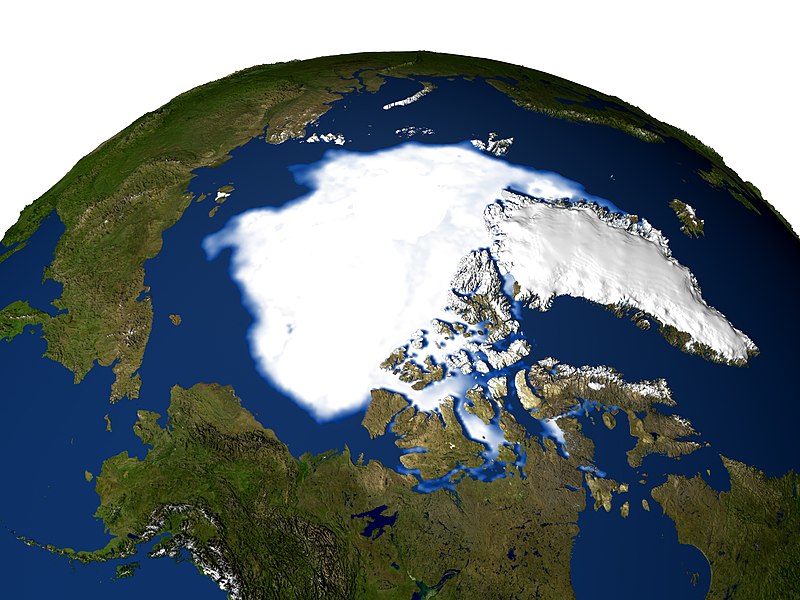
2005 NASA Sea Ice extent Imagery. (Source) – Wikimedia Commons – NASA
Anyway, this new paper entitled “Arctic sea-ice decline archived by multicentury annual resolution record from crustose corraline algal proxy” recently appeared in PNAS. In this study the authors used corralline algae as a new proxy to estimate sea ice coverage in the Arctic. The question that these authors sought to answer using corraline algae as a proxy was: can we calculate past sea ice coverage and can we then use the larger knowledge base we now have about past sea ice to apply that to predicting future sea ice conditions given at current models are not very reliable at predicting future sea ice coverage?
First, lets look at this corraline algae proxy. Corraline algae is a type of red algae that have been around since Cretaceous. As the name suggests they tend to be red in colour and often grow in coral reefs. According to Wikipedia appear as “pink to pinkish-grey patches, splashed as though by a mad painter over rock surfaces”. (How poetic eh?). Anyway, they are widely distributed globally and occur in all the world’s oceans up to the maximum depth light can penetrate as they are photosynthetic and their growth depends on light and temperature. The species of corraline algae used in this study was Clathromorphum compactum, which forms a new layer ever year, much like a tree forms rings. Clathromorphum is an encrusting variety of red algae that grows on rocky substrates year after year essentailly in perpetuity as the only thing that can prevent it from adding another high Mg calcite later is if something actually breaks it apart or eats it. The authors found samples of Clathromorphum up to 646 years old!

Photo of coralline algae – Wikimedia Commons – Author: Derek Keats
.jpg)
The way a proxy works is that a certain feature of the sample, such as its chemistry or growth ring width, can be used to tell us about conditions that were responsible for chemical changes in the sample or the size of its growth rings. It is even better if the sample can be used to represent large time periods. Therefore a sample of 646 year corralline algae has the potential to be used as a proxy if its chemical or growth features are caused by a change in living conditions. As it happens the growth of corralline algae is directly related to amount of sun in receives. For example, if it is very sunny the algae will have larger growth rings, if it is not sunny the algae will have very small growth rings. Furthermore, when the algae is growing it preserves the Mg/Ca ratio of the seawater it is growing in inside its calcite skeleton. However, if the algae is not growing the recording of Mg/Ca ratios stops. So, if there is no sea ice the algae makes thicker growth rings and has a high Mg/Ca ratio, when there is sea ice covering the area the algae is growing in the growth rings are small and the Mg/Ca ratios are low. The fact that coralline algae has two proxies that can tell us about sea ice conditions makes it an excellent tool for looking into the past to see ice coverage. It is a great double whammy!!

Fig. S2. Analytical reproducibility. Annual cycles of Mg/Ca ratios measured by electron microprobe (A) on two parallel transects along main axis of growth on uppermost 5 mm of sample Ki2 (B). Microscope image of polished sample shows ∼80 annual growth increments. Cycle shapes in A are characteristic of break in growth during sea-ice season, with narrow downward pointing peak. Summer portions of cycles instead are smooth, reflecting summer light and temperature cycle patterns following spring breakup of sea ice. Note similarity of winter Mg/Ca ratios reflecting constant seawater temperature under sea ice. Sample spacing, 15 μm (average annual growth of Ki2 = 172 μm) results in average resolution of ∼11.5 samples per year. Mg/Ca ratios are based on atom percent of Mg and Ca. Photo and caption used in accordance with PNAS guidelines for educational purposes only.
So, based on the fact that the size of the growth rings and Mg/Ca ratios in the growth rings of Clathromorphum tell us about sea ice coverage the authors set out to sample Clathromorphum from a variety of locations around Northern Canada. What they found is pictured in the figure below, but I’ll cover the highlights.
1. The record of sea ice coverage obtained from the coralline algae proxy agrees well with known sea ice coverage data from the 1970’s onwards.
2. The algal proxy shows that sea ice coverage has been declining steadily for the past 150 years, the latter part of which agrees with actual observations of sea ice coverage.
3. A 646 year record shows that sea ice coverage was high between 1530 and 1860, which corresponds to the Little Ice Age.
4. The results from this proxy agree well with those from other proxies such as ice cores and anthropological evidence for high sea ice coverage during the Little Ice Age.

Fig. 3. Algal proxy record (red) compared with observational (blue) and proxy (green) data (see Methods for detail on records). Gray lines represent 5-y moving average and colored lines, 15-y low-pass filtered (Savitzky–Goley) annual data. Algal proxy time series plotted on inverted scale to indicate declining ice cover. Light gray bars show periods of positive algal anomalies, reflected by negative ice anomalies in observational records, and positive δ18O ice core excursions. Linear trends for all time series are plotted from 1850 onwards. All individual algal specimens yield similar trends (Fig. S3). RC indicates position of radiocarbon analyses. Values are 2σ calibrated results (Table S1); all values fall well within age model derived from growth increment counting.
So there it is. Coralline algae is a great new proxy for sea ice coverage. I am left wondering a few things about the use of this proxy that hopefully the authors will address in future work. The foremost question in my mind is: could this be used as a proxy for sea ice coverage into the distant past? We find a lot of coralline algae in the fossil record so perhaps if the paleo-latitude was known, these preserved specimens could be used to interpret sea ice conditions thousands or even millions of year ago? What do you think? I’m not sure how well Mg/Ca ratios are preserved, but the growth rings certainly are….
Halfar J., Adey W.H., Kronz A., Hetzinger S., Edinger E. & Fitzhugh W.W. (2013). Arctic sea-ice decline archived by multicentury annual-resolution record from crustose coralline algal proxy, Proceedings of the National Academy of Sciences, 110 (49) 19737-19741. DOI: 10.1073/pnas.1313775110
The article that first called my attention to this paper.
Glenn Hall
Good article. This is pretty important stuff. I caught the article in PNAS: Glad other people did too.
Given the size of the systems, the time frames involved, solar cycles, Milankovitch cycles, volcanic activity, etc., it is hard to assess “baseline” climactic changes over time and attribute them (or their percentage of contribution) to particular source. This appears to offer a remarkably precise proxy (given inherent impression involved with proxies) for Arctic ice extent.
I’m hoping that Arctic ice proves to be a good proxy for total heat content of the oceans, which doesn’t seem totally unreasonable . . . . Since it looks like we are finally getting a better handle on ocean temps with ARGO being fully deployed (still far too little, too shallow, and too variable for my taste), hopefully we will be able to get some nice calibration on the various systems, their interplay, and the models they are using.
By the way, I read and really liked your Radon article too– but the link and the house points of entry have gone stale unfortunately. Radon is a very real health risk. I think it is a great service to provide as much info about it as possible. One negative aspect about the energy conservation stuff is that people have buttoned up their houses– preventing outside air exchange. Add to that the vacuum effect that central AC and heat can have– well as you would expect the government (or at least the U.S. government) didn’t figure out that all those energy efficiency subsidies it was offering might be a problem until long after much of the work was done. And, being the U.S. government, it didn’t step to the plate and say “Wait. We may have screwed up. You need to check you home . . . . ” Radon can also be present concentrations warranting attention even in areas with bedrock that would seem to present little problem. Perhaps that is due to underlying shale or something.
Really liked the decay chart–hadn’t ever seen that before.
Also, liked your article on hydraulic fracturing. The main environmental problem with hydraulic fracturing is the potential use of large amounts of potable surface water and proper management of the frack fluids on flowback. These are not anything earthshaking, to say the least. All produced waters should always be properly managed. Lots of companies are starting to recycle and look at recycling fluids. There are even companies that do fractures using LPG — which I think is pretty smart, although there is perhaps a tad more risk involved. The industry, however, generally knows how to manage that kind of risk well.
It is, of course, always critical that wells be properly designed, have surface casing to an adequate depth, and be properly cemented. That, however, is nothing new.
I think the big “environmental” debate over massive hydraulic fracturing has ever so much more to do with the process of producing oil and gas in that manner and where that is occurring (i.e., Pennsylvania) than it does over any actual environmental issues. Folks in Texas and North Dakota aren’t real worked up over it.
I also see concern over global warming as an ancillary driver, which I consider most unfortunate: The environmental movement would be much stronger if they considered their real concerns and how to be credible and effective in getting those addressed. I do, however, think the standards related to fugitive methane emissions need to be tightened some too. The biggest problem there, however, isn’t going to be at the wellhead: It will be the midstream and most especially the residential distribution that are the big culprits on fugitive methane emissions. Of course, as you know, usually we are just speeding the route of methane to the surface: no trap or confining layer is perfect and there are continuous emissions of it from deposits all over the world.
Thanks for the cool stuff.
Matt Herod
Thank you so much for your excellent comment and support Glenn.