Aerosols dominate the uncertainty in the total anthropogenic radiative forcing. A complete understanding of past and future climate change requires a thorough assessment of aerosol-cloud-radiation interactions.
This is one of the conclusions about aerosols and their impact on our climate from the the final report from the Intergovernmental Panel on Climate Change (IPCC) on the physical science basis that was released recently. What brought them to this conclusion and what does it mean? In this piece, I’ll go through the headline statements and findings.
The IPCC are concerned with assessing how various factors affect the Earth’s climate and it dedicates an entire chapter to aerosols and clouds, which is accessible here.
How do aerosols impact our climate?
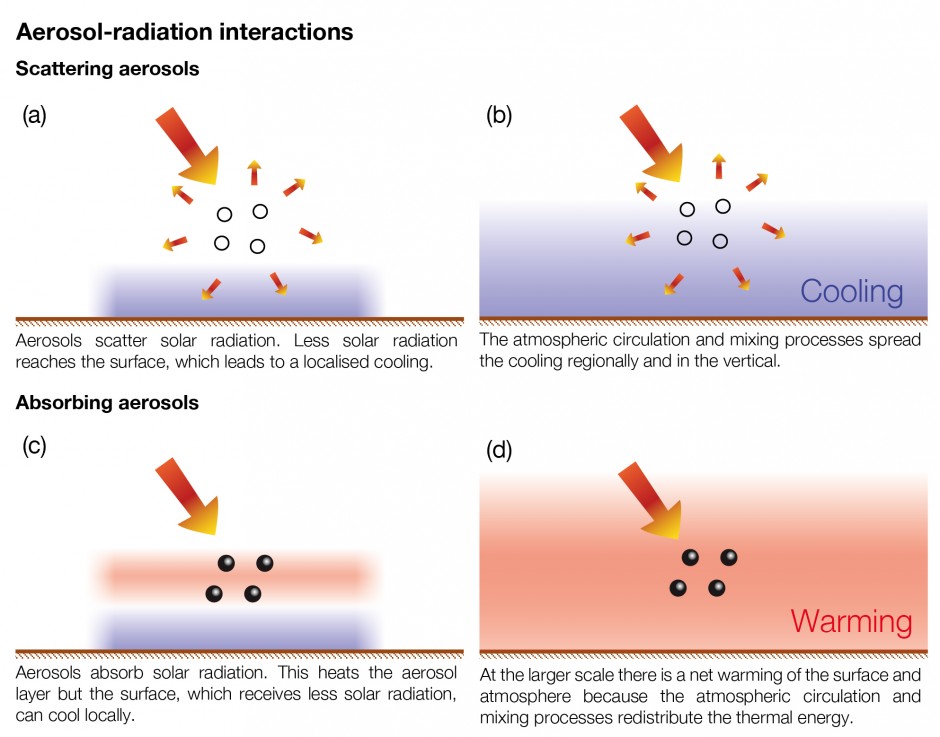
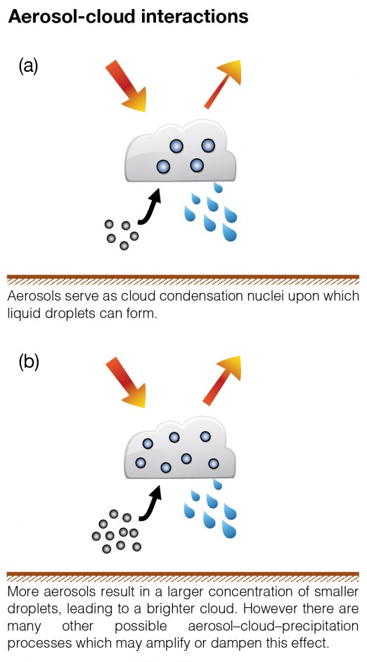
Aerosols, can broadly influence the climate in two ways; aerosol-radiation interactions and aerosol-cloud interactions. The IPCC included some nice diagrams of how these processes occur, which I’ve included below.
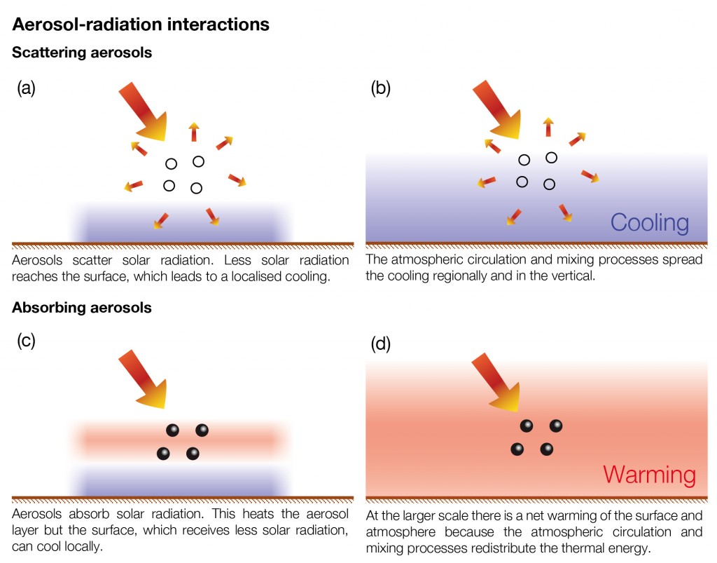
Illustration of aerosol-radiation interactions produced by the IPCC. This figure and more are available here.
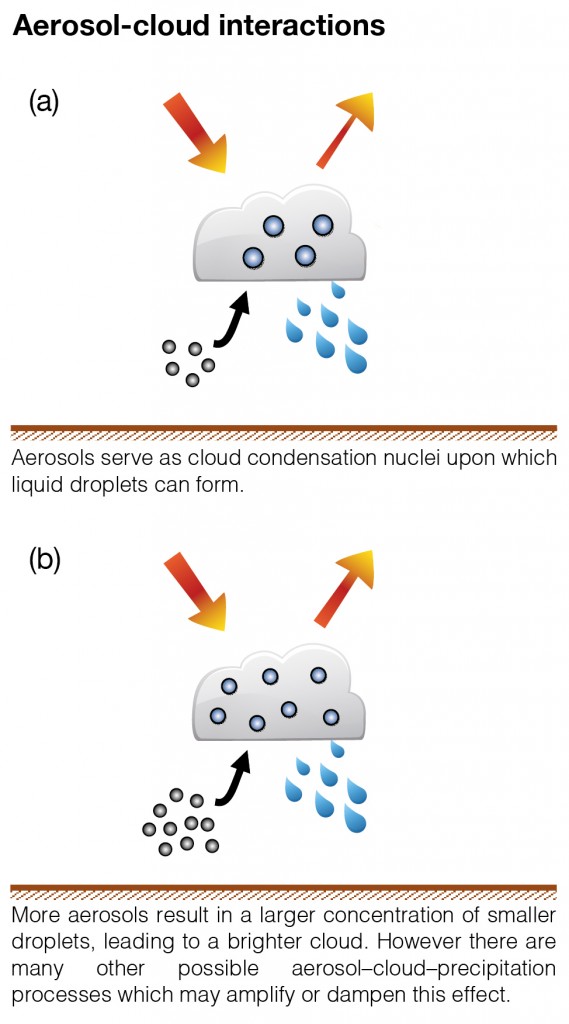
Illustration of aerosol-cloud interactions produced by the IPCC.
Both of these interactions are well established but the problem is pinning down the magnitude of these effects at larger scales and over time.
Headline numbers
The IPCC often refer to a term known as radiative forcing when assessing climate impacts. This illustrates the change in the amount of incoming versus outgoing radiation to our atmosphere. This regulates global temperatures and can affect things like circulation patterns and precipitation. Positive radiative forcing values increase temperature, while negative values reduce them. This value is usually referenced back to before the Industrial Revolution (typically 1750), when human influences on the composition of the atmosphere were more limited.
To put this in some context, the radiative forcing for carbon dioxide is 1.82 W/m2, with a reported range from 1.63 to 2.01 W/m2. What this means is that since 1750, adding carbon dioxide to our air has altered the radiation balance of the atmosphere and that this will cause a warming in the absence of any cooling factors.
In the table below, I’ve collated the various estimates for the aerosol influence from the report. As well as the central estimate, it is important to examine the range as this is one of the crucial aspects that drives the statements about our uncertain understanding of aerosols. The central estimates and the forcing range all suggest that aerosols exert a cooling influence on our climate; aerosols offset some of the warming influence from carbon dioxide and other greenhouse gases. If we first focus on the IPCC 2007 and 2013 values, we see that the central estimate has for the latest report (AR5) indicates that aerosols are exerting less of a cooling effect than estimated previously. The range of the forcing estimate has also reduced.
The IPCC is effectively saying that the cooling influence from aerosols is slightly weaker than previously estimated and that our understanding has improved.
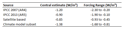
Aerosol radiative forcing estimates.
The other values refer to different ways of calculating the impact and it is these numbers that inform the overall value in the report. The satellite based value refers to studies where satellite measurements of aerosol properties are used in conjunction with climate models; they are not wholly measurement based. In terms of studies using climate models on their own, the IPCC used a subset of climate models for their radiative forcing assessment, choosing those that had a “more complete and consistent treatment of aerosol-cloud interactions”.
The satellite based central value of -0.85 W/m2 is less negative than the central value from the climate models, which means the models indicate more cooling than the satellite based estimate. Compared to the subset of climate models that the IPCC used for their radiative forcing judgement, there is little overlap between their ranges also.
Why so uncertain?
This lack of agreement is a big driver for the large uncertainty range. It’s important to stress that there isn’t a strong reason to “trust” one set of results over another here as both satellite observations of aerosol properties and their representation in climate models are prone to many biases and it isn’t currently clear how these will impact the results.
Both methods are very sensitive to the assumed pre-industrial conditions assumed by the studies. Both methods have difficulties dealing with clouds but for different reasons.
Satellites can’t typically see through clouds, so they can miss aerosol trapped below them. Another major challenge is when layers of aerosol exist above clouds, which can affect the satellite measurements. Satellites are best suited to measuring the total amount of aerosol in the atmosphere. They have difficulty identifying different aerosol types, which means they can lump together natural and anthropogenic aerosols. They also have difficulty determining the relative importance of scattering or absorbing aerosols, which will determine the climate impact. Typically they can’t determine where the aerosol is in the vertical dimension of the atmosphere, which again will influence the climate impact. There are certainly advances in these areas but as ever, more work is required.
Models on the other hand, have difficulty representing aerosol-cloud interactions due to cloud systems typically being smaller than the resolution of a climate model, the complex number of processes at play and the lack of real-world measurements to test them. There is some evidence to suggest that climate models at the global scale tend to overestimate the size of the aerosol effect on cloud properties.
If we examine more details from the climate models, we see that there are large differences between models in terms of what types of aerosol it considers to be important. For example some models say that dust is a major contributor to the global aerosol burden, while others disagree. These are important details as climate models can sometimes broadly agree in terms of the radiative forcing estimate they provide but for very different reasons. Black carbon is another species that can contribute to varying degrees in different models, which is important as it warms the atmosphere; how a model represents black carbon is going to have a strong influence on the reported cooling. Nitrate is a potentially important species that often isn’t even included in climate models.
To summarise: it’s complicated.
What does this mean for climate change?
The short answer is: probably not a lot.
The change from the previous report is overall quite small (0.3 W/m2) and this is predominantly a result of improvements in our ability to represent aerosol processes (particularly clouds) since the last report. To put the change in context, between 2005 and 2011, the radiative forcing by greenhouse gases increased by 0.2 W/m2 due to increased concentrations in our atmosphere alone. At present, the uncertainties in aerosol radiative forcing mean that making definitive statements are likely unwise and putting faith in any one particular result will be fraught with difficulties. Focussing on the global scale also ignores the much larger regional impacts that aerosols can have, which is of more relevance to the wider issue.
The current state of understanding of aerosols suggests that they’ve exerted a cooling influence on our climate, which has offset some of the warming expected from the increase in greenhouse gases in our atmosphere. Improving this understanding will be crucial for assessing both past and future climate change.