Climate change

What’s Geology got to do with it? 2 – Coffee

Flo Bullough October 24, 2013

We should start this post with a declaration of interest. We absolutely love coffee. Whether it’s latte, macchiato, flat white (or cafe au lait for Marion!) we drink it everyday! So for our second installation of “What’s geology got to do with it?’ we’re going to highlight the connections between coffee and geology!

Coop loves his coffee! Source

As well as being absolutely delicious (and often powering an entire community of researchers, PhD Students, lawyers etc through work on a daily basis!) coffee is the 2nd most traded commodity in the world, sitting in a list dominated by other commodities important to geoscience!

Crude Oil
Coffee
Cotton
Wheat
Corn
Sugar
Silver
Copper
Gold
Natural Gas

Coffee and Soils!

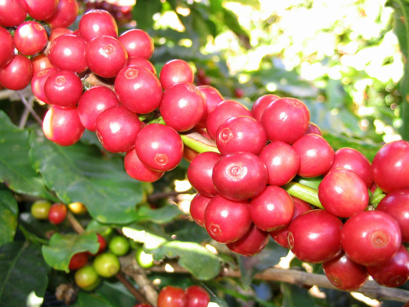
Coffee berries, a variety of Coffeea Arabica. Source – Marcelo Corrêa, Wikimedia Commons.

In order to supply the international demand for coffee, coffee trees require a large supply of nutrients. These nutrients are delivered through soils which are ultimately formed from the breakdown and erosion of rocks. In addition to allowing coffee trees to grow, the soil makeup will also contribute to a coffee’s unique flavour profile. Having said that, the combination of factors affecting taste is so complex, that even from a single plantation you can find variation in quality and taste.

What does coffee need to grow?

Aside from cool-ish temperatures (~20 degrees) and high altitude (1000-2000 metres above sea level), Coffee requires a wide variety of essential elements in order to grow and deliver the delicious stuff we drink. These elements are delivered through the soil profile. The usual suspects like Phosphorus, nitrogen, potassium, calcium, zinc and boron are all very important. The level of potassium influences total sugar and citric acid content while nitrogen is important for amino acid and protein buildup and can influence caffeine build up. Boron is important for cell division, cell walls and involved in several enzyme activities. It also influences flowering and fruit set and affects the yield. In addition to soil type and content, factors such as slope angle (15% is optimal), water supply (good supply with interspersed dry periods are essential) and altitude exert strong influence on the success of coffee growth.

What soils are best?

Coffee can be grown on lots of soils but the ideal types are fertile volcanic red earth or deep sandy loam. For coffee trees to grow it is important that the soil is well draining which makes heavy clay or heavy sandy soils inadequate. Some of the most longstanding and famous coffees are grown on the slopes of volcanoes or in volcanic soil, also known as ‘Andisols’.

Definition of Andisol (USDA soil taxonomy) – ‘Andisols are soils formed in volcanic ash and defined as soils containing high proportions of glass and amorphous colloidal materials, including allophane, imogolite and ferrihydrite.’

Coffee grows on the slopes of these volcanoes in El Salvador. Source – NASA, Wikimedia Commons

But why are they so fertile? This is due to how young, or immature they are as soils. They still retain many of the elements that were present during the formation of the rock, they haven’t been plundered over hundreds of years of agriculture, they haven’t undergone extensive leaching and are relatively unweathered. This means they often include basic cations such as Mg, Ca or K (which can be easily leached out) and often retain a healthy supply of trace elements. Whilst these soils are very fertile, they only cover around 1% of the ice-free surface area of the earth. They can usually support intensive use for growing coffee and other mass crops such as maize, tea and tobacco. Despite the high fertility of volcanic soils, many do need a nutrient top-up during the growth cycle that comes from natural manure or fertilisers, which are themselves in diminishing supply.

Volcanic soils also have a good structure and texture for coffee growth as they often contain vesicles, which makes them porous and ideal for retaining water. Shallow groundwater is bad for coffee growing as it can rot the roots and it needs to be at least 3 metres deep. Roots of coffee have a high oxygen demand so good drainage is essential.

Where does coffee grow and why?

It is no surpise then that some of the most famous and historic coffee growing regions are in areas of past and current volcanic activity such as Central America, Hawaii and Indonesia. Coffee trees produce their best beans when grown at high altitudes in a tropical climate where there is rich soil. Such conditions are found around the world in locations along the Equatorial zone.
Coffee is grown in more than 50 countries around the world including the following;

Hawaii – coffee is grown in volcanic soil or directly in the loosened rock. The location and island climate provides good growing conditions.
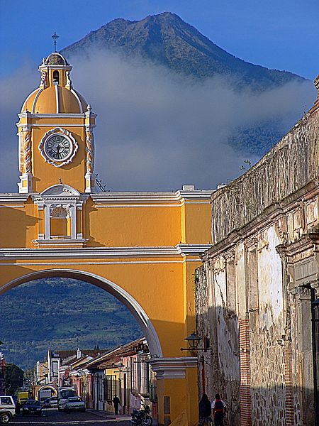
Volcán de Agua overlooking Antigua in Guatemala an area with a big coffee production industry. Source – Zack Clark, Wikimedia Commons.
Indonesia – coffee production began with the Dutch colonialists and the highland plateau between the volcanoes of Batukaru and Agung is the main coffee growing area. Ash from these volcanoes has created especially fertile andisols.
Colombia – thought that Jesuits first brought coffee seeds to South America. One of the biggest producers in the world, regional climate change associated with global warming has caused Colombian coffee production to decline since 2006. Much of the coffee is grown in the cordilleras (mountain ranges).
Ethiopia – grown in high mountain ranges in cloud forests.
Central America – rich soils along the volcanic range through central america, equatorial temperatures and mountainous growing areas make this a powerhouse in the coffee growing world.

Coffee and Climate!

Like many crops and food commodities, good coffee requires good climate. For our favorite bean, this typically means temperate regions at altitudes of 1000-2000 m. But climate is changing and this is likely to have a big impact on coffee growth, and by association, on the livelihood of millions of local coffee farmers who rely on its production.

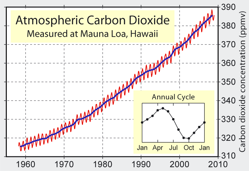
In its latest report out last month, the UN’s Intergovernmental Panel on Climate Change (IPCC, the leading body assessing climate change impacts) confirmed for the 5th time what climate scientists worldwide already know: that our climate is warming as a result of human activities. Global temperatures have already risen by almost 1C since the end of the 19th century and will continue to rise at even faster rates over the coming century.

There are two ways in which a changing climate will impact coffee growth and production.

First, increasing temperatures or changes in precipitation will directly affect the areas suitable for coffee growth, leading to a loss in coffee growing environments.

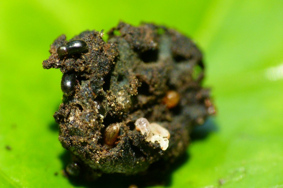
A coffee berry being chewed up by hungry Hypothenemus hampei – Source: L. Shyamal, Wikimedia Commons.

Second, and perhaps most importantly, changing climate and higher temperatures will affect a little insect called Hypothenemus hampei (H. hampei for short). H. hampei is small but lethal. This beetle-like insect is what people call a coffee berry borer. It is the most important threat to coffee plantations worldwide.

Born in central Africa, H. hampei began colonising coffee plantations worldwide with the global movement and commerce of coffee beans. H. hampei likes warm climates. Until about a decade ago, it was very happy munching away at low-altitude beans, below the preferred altitude of our beloved Arabica coffee (between 1200-2000 m in East Africa).

But with rising temperatures, the berry borer can now survive at higher altitudes. On the slopes of Mt Kilimanjaro in Tanzania, H. hampei has climbed 300 m in 10 years.

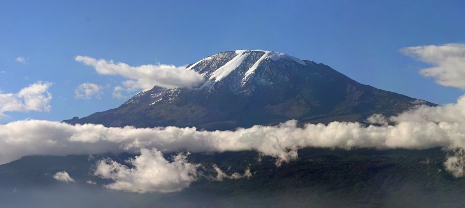
Mount Kilimanjaro – Source: Muhammad Mahdi Karim, Wikimedia Commons.

H. hampei causes over $500 million loss annually in East Africa alone. The borer is gaining both geographical extent (it is only absent from coffee plantations in China and Nepal, having infiltrated Puerto Rico in 2007 and Hawaii in 2010) and altitude. A further 1C increase will see the borer develop faster and gain new territories.

The Colombia coffee belt – Source: Instituto Geografico Agustin Codazzi, Wikimedia Commons.

In Colombia, where coffee accounts for 17% of the total value of crop production, temperatures in the coffee belt region are projected to rise by 2.2C by 2050. This could both shorten the coffee growing season and allow the pest to make its way above 1500 m.

It has been estimated that Colombian plantations would have to be moved up by 167 m for every degree of warming.

In East Africa, studies predict that Arabica coffee, currently grown at 1400-1600 m, will have to shift to 1600-1800 m by 2050 as a result of rising temperatures.

But it is unlikely that East African coffee plantations will be able to adapt. For one, suitable high altitude habitats are not common. Second, population growth is likely to put a huge demographic pressure on arable land (the population in Ethiopia is set to double by 2050 – see this fact sheet by the Population Reference Bureau) and it is likely that the shrinking available arable land will be used to cultivate other crops over coffee.

The impact of climate change on invasive pest species is something that ecologists are studying worldwide. Small changes in average temperatures can have huge bearings on where these pests live and what they feed on, and this seems to already be the case for the coffee berry borer.

Let’s hope Flo and I can continue enjoying our weekly Four Degrees coffee meetings for many years to come!

Flo and Marion

Climate change: it’s just a matter of time!

Marion Ferrat September 20, 2013

Natural or man-made: what factors are responsible for the climate changes we are seeing today? Ahead of the release of the latest IPCC report next week, Marion Ferrat discusses the different factors affecting climate change and shows that who takes the blame all depends on timing…

Over the past century, our planet’s climate system has been changing. Changes in the composition of the atmosphere, holes in the ozone layer, warming temperatures and sea level rise are only some of the factors that have been observed worldwide.

Earth taken by the crew of the Apollo 17 spacecraft – Source: NASA, Wikimedia Commons.

A fixed observer looking at our planet for the past few billion years would have seen patterns of warming and cooling of its surface, ice sheets growing to the tropics or shrinking to the tips of the poles, deserts forming, seas drying, oceans overturning and vegetation changing. So who is to blame for our current changing climate? Is climate change natural or man-made?

What factor is most important in driving climate change really depends on the timescale you consider. So let’s take a short journey through climate space and time to shed more light on who is to blame for climate change.

The million-year climate change: blame the continents
The hundred thousand-year climate change: blame the Sun
The thousand-year climate change: blame the climate!
The 21st century climate change: blame ourselves

The million-year climate change: blame the continents

The Earth’s climate history is divided into primary climate periods, millions of years long, of increase or decrease in the temperature of the Earth’s surface and atmosphere. These periods are referred to as Greenhouse Earth and Icehouse Earth (or Ice Age), respectively.

Fictional representation of a ‘Snowball Earth’ – Source: Neethis, Wikimedia Commons.

The main characteristic of an Ice Age or Icehouse world is that permanent ice sheets are present at the surface of the Earth. The thick ice sheets covering Greenland and Antarctica today mean that we are currently living in an ice age, which began 2.6 millions of years ago.

In a Greenhouse world, on the contrary, ice sheets and glaciers are absent from the surface of the Earth. At the height of these times, carbon dioxide levels in the atmosphere can vary between a few to a few hundred times their present level.

The exact causes behind shifts between greenhouse and icehouse worlds are still debated but scientists agree that two factors play an important role: the position of continents at the surface of the Earth and the concentrations of greenhouse gases (mainly CO2 and methane) in the atmosphere.

Animation of the breakup of Pangea – Source: USGS, Wikimedia Commons.

The position of the continents and oceans is important in driving the million-year-long climate cycles as it has a huge influence on atmospheric composition and oceanic flows (see this cool animation showing the movement of the British Isles over geological time!). For example, the grouping of continents in particular places can stop the flow of warm water from the equator to the poles and cool down polar water, until ice sheets begin to form.

Eruption column rising from the east Ukinrek Maar crater in Alaska - Credit: R. Russell/USGS, Wikimedia Commons.

Eruption column rising from the east Ukinrek Maar crater in Alaska – Source: R. Russell/USGS, Wikimedia Commons.

Plate tectonics can also drive climate change by influencing the concentration of CO2 in the atmosphere. The presence of large volcanoes can play an important role in driving long-term shifts from an icehouse to a greenhouse world because extensive volcanism can release large quantities of greenhouse gases into the atmosphere. Once enough CO2 builds up, the greenhouse effect kicks in and acts to warm the planet, pulling it out of its million-year ice age.

Once an initial change is triggered, the climate system will act to amplify it internally until the switch between ice and greenhouse world is complete.

The hundred thousand-year climate change: blame the Sun

Overlain on top of the huge greenhouse or icehouse periods are shorter, regular periods of climate change.

Over timescales of tens to hundreds of thousands of years, the Earth undergoes cycles of cooling and warming, driven primarily by small changes in the amount of energy received from the Sun. These periods are known as glacial and interglacial cycles, i.e. times within an ice age when the Earth is colder or warmer than average. We are currently living in an interglacial period called the Holocene, which began roughly 11,000 years ago.

An example of changes in eccentricity.

Glacials and interglacials are driven by what we call orbital changes: small changes in the Earth’s orbit, which alter the amount of solar energy received at the Earth’s surface. These changes are cyclical and known as Milankovitch cycles, after the Serbian astronomer who first recognised them during the First World War.

Obliquity or axial tilt – Source: Dna-webmaster, Wikimedia Commons.

There are three types Milankovitch cycles. The first, called eccentricity, is linked to the shape of the Earth’s orbit around the sun. The orbit changes from the shape of a circle to that of an ellipse over average timescales of roughly 100,000 years. When the orbit is more elliptical, the Earth is either closer or further away from the Sun than when the orbit is circular, driving changes in the amount of solar energy received at the surface. Climate data for the past 800,000 years show that ice sheets have grown and shrunk roughly every 100,000 years, likely driven by changes in eccentricity.

Precession of Earth’s rotational axis due to the tidal force raised on Earth by the gravity of the Moon and Sun – Source: NASA/Mysid, Wikimedia Commons.

The second type is linked to changes in the Earth’s axis. The Earth rotation axis is tilted; this tilt is largely what drives our seasons. The amount of tilt (or obliquity) also varies with time, over periods of roughly 41,000 years.

Finally, if one could watch the Earth from a fixed star in the universe, they would see its axis rotating slightly, a little bit like the wobble of a spinning top as it slows down. This is called precession and changes over periods of roughly 23,000 years.

The 100,000, 41,000 and 23,000-year Milankovitch cycles alter the amount of sunshine received on Earth and drive many changes in the Earth’s climate on these timescales, as has been observed in temperature and CO2 records.

The thousand-year climate change: blame the climate!

X-ray photo of surface sediment (0-25 cm) from the Southern Ocean with scattered gravel as ice rafted debris – Source: Hannes Grobe/AWI, Wikimedia Commons.

In the last decades of the 20^th century, scientists began to find clues in the geological records of the North Atlantic Ocean and Greenland ice sheet that climate change was also occurring at higher frequencies than those linked to orbital and tectonic cycles.

Icebergs contain plenty of eroded rock and sediment. When they break-off into the ocean and melt, much of this material falls to the seafloor and can be seen as anomalies in the geological record called ice-rafted debris. Ocean cores revealed that thousand-year pulses of such debris could be found regularly throughout the past 100,000 years, suggesting rapid periods of iceberg break-off and discharge of cold water to the North Atlantic Ocean.

The Greenland ice cores also revealed that periods of rapid warming followed by slow cooling were occurring every few thousand years. These events seem to occur roughly every 1,500 years, though precise dating on these timescales can be difficult.

Such events are known as millennial cycles and are what scientists refer to as ‘abrupt’ climate change.

Similar changes have since been recognised in many locations, including the north Pacific Ocean and the tropics, suggesting that changes can be rapidly transferred between different regions of the globe by the climate system itself. One possible mechanism is that large bursts of cold water in the North Atlantic Ocean could alter the global circulation of ocean currents, which is largely driven by density changes in the North Atlantic region.

The global circulation of the oceans, known as the ‘conveyor belt’ – Source: Thomas Splettstoesser, Wikimedia Commons.

The 21st century climate change: blame ourselves

So Earth’s climate has changed drastically throughout the course of its history, driven by external factors such as changes in the Earth’s orbit and internal factors such as tectonics and physical connections between different parts of the climate system. Yes, these climate changes are natural and, yes, temperatures and CO2 have at multiple times been higher than they are today.

However, there are a few points worth making:

Smog over Beijing, China.

#1 – The most drastic changes have occurred very slowly, on timescales of hundreds of thousands to millions of years. These are thousands of orders of magnitude larger than that of a human life;

#2 – At all scales, atmospheric CO2 concentrations have played a huge role in climate change, contributing largely to the greenhouse effect, affecting ocean composition and acidity and being a crucial component of plant and animal life cycles;
#3 – Until the start of the industrial revolution, humans in our modern societies have evolved and lived through relatively stable climate conditions , with stable CO2 concentrations between 260-280 parts per million (ppm) for the past 10,000 years;
#4 – CO2 levels have constantly increased since the industrial revolution due to human emissions. A record global atmospheric CO2 concentration of 400 ppm was observed in May 2013 at the Hawaiian Mauna Loa observatory. This is the highest CO2 level in over 800,000 years, higher than any other interglacial period during this time.

Atmospheric CO2 during the past 417,000 years (417 kyr). Blue: CO2 records from ice cores drilled at the Vostok station in Antarctica; Red: CO2 increase to 380 ppm between 1800 and today due to anthropogenic emissions from fossil fuels- Source: Hanno, Wikimedia Commons.

Atmospheric CO2 during the past 417,000 years (417 kya). Blue: Records from ice cores drilled at the Vostok station in Antarctica; Red: CO2 increase since 1800 due to anthropogenic emissions from fossil fuels – Source: Hanno, Wikimedia Commons.

The speed at which this human-induced rise in CO2 has occurred is worrying, increasing by nearly a third in just over 150 years.

The climate system will adjust to these changes over the next centuries as it has in the past. But the real issue is that these adjustments will not be in line with our modern inhabited world. As millennial cycles have shown, polar changes can be transferred between different regions of the Earth in ways that we still do not fully understand. Humans as a whole will likely adapt to future climate repercussions but particular vulnerable regions and communities will not.

Atmospheric CO2 concentrations measured at Mauna Loa, Hawaii - Source: Robert A. Rohde, Wikimedia Commons.

Atmospheric CO2 concentrations measured at Mauna Loa, Hawaii, since 1960 – Source: Robert A. Rohde, Wikimedia Commons.

Modern climate change is not a case of the end of the world but more of the end of the world as some people know it. Small islands and low-lying regions will suffer, so will areas affected by unpredictable droughts or floods.

By contributing in such an excessive way to concentrations of atmospheric CO2, humans are to blame for the climate changes we will continue to see in coming decades and even centuries; and not all of us will be able to adapt to it.

What’s Geology got to do with it? 1 – The Maya civilisation

Flo Bullough August 30, 2013

Tikal Mayan ruins in Guatemala. Credit - chensiyuan, WIkimedia Commons.

Geology is not just about looking at rocks. From finding oil and gas and tackling climate change to manufacturing, archaeology or geopolitics, geoscientists appear in most spheres of today’s world and economy, albeit often behind the scenes. In a new series of posts we will be looking at how geology relates to interdisciplinary or seemingly unconnected topics, which, at first glance, might seem like they have nothing to do with geology at all.

Earlier this year, Iain Duncan Smith (UK Work and Pensions Secretary) had a well publicised clash with geologists after saying in an interview on the Andrew Marr show regarding the legal battle of Cait Reilly – “The next time they go into their supermarket, they should ask themselves this simple question, when they can’t find the food they want on the shelves – who is more important – the geologist, or the person who stacked the shelves?” (see this excellent press release from the Geological Society in response). In way of response to this comment, this series will focus on the links between geology and the wider world and the importance of approaching problems from an interdisciplinary perspective. We hope to highlight the extensive reach of geology and how it can enrich our understanding of topics far outside of the traditional subject area.

1. The Maya civilisation

For our first post in the series we have chosen to look at the pre-Columbian Maya Civilisation, partly inspired by a recent story on the discovery of a large Mayan sculpture in a Guatemalan archaeological site .

Tikal Mayan ruins in Guatemala. Credit – chensiyuan, WIkimedia Commons.

The Maya Civilisation can be traced as far back as 2000 BC and occupied southern Mexico and northern Central America (including the modern territories of Guatemala, Belize and Honduras). It prospered until 900 AD and continued until the arrival of the Spanish. Their golden age between 300 and 900 AD is a period characterised by flourishing art and architecture as well as developments in mathematics and astronomy. Mayan cities are dotted throughout Central and South America, the more famous sites include Chichen Itza and Palenque in Mexico and Tikal in northern Guatemala (see this map of the geography of the Mayan civilisation).

So… How does geology relate to this great civilisation? Elements of geology came into the daily lives of the Mayans in many forms through their building materials, the siting of their cities and the materials and minerals they used for trading, building infrastructure and creating objects used in their everyday lives. Climate change may also have greatly influenced the Mayan people and is thought to have led to both the expansion and the disintegration of this civilisation. We take a look at these different aspects below.

Siting of Mayan cities

The name of the city ‘Chich’en Itza’, located in Mexico, means ‘At the mouth of the well of Itza’. This refers to its location close to several ‘Cenotes’ (or in English, sink-holes). Sinkholes are cavities in the ground, often in limestone formations, caused by water erosion – these have received a lot of press recently due to their building swallowing activity! Find out more about sinkholes here. It’s thought that Cenotes provided access to the underworld, due to the discoveries of skeletons in sinkholes and caves near to archaeological sites. The cenotes were also fed by underground rivers, which provided water for the population.

Cenotes at Chichén Itzá, Yucatán Peninsula, Mexico. Credit – Emil Kehnel, Wikimedia Commons.

Building and Architecture

Mayan cities grew by using sacbeob (white roads, or limed causeways) to connect great plazas and temples. These were made from limestone due to its ease of handling and local availability. Stone for buildings was taken from local quarries. Limestone was preferentially used because it was easy to remove using the stone tools available and because it could be used to make mortar through crushing and burning. Limestone was also used for both mortar and stucco.

Agriculture and Natural Hazards

Map of Guatemala volcanoes. Credit – USGS, Wikimedia Commons.

One might expect a civilisation that prospered over a long period of time to have developed a thriving agriculture to meet the needs of an expanding population. But limestone is the dominant rock type in the area and does not usually generate good soil. Many Mayan cities are therefore believed to have had poor soils which puzzled scientists and archaeologists as to how they could sustain such great cities.

In a recent article in National Geographic, it was suggested that volcanic ash had been ‘spectacularly important’ in Mayan agriculture. Recently scientists discovered a distinct beige clay mineral, a type of smectite (the same mineral recently found on Mars!), in ruined canals at Guatemala’s Tikal archaeological site—once the largest city of the southern Maya lowlands. Chemical fingerprinting techniques were used to show that the smectite at Tikal didn’t come from dust carried over from Africa by air currents as previously thought but from volcanoes within what are now Guatemala, El Salvador, Honduras, and Mexico. The volcanoes in this region are produced by subduction of Pacific oceanic crust beneath the North American and Caribbean Plates. Volcanoes also brought their fair share of disaster to the Mayans. A village in El Salvador was completely buried when the nearby Ilopango volcano erupted in the 6^th century A.D, not unlike the more famous Mt Vesuvius eruption in 79 AD, which buried the cities of Pompeii and Herculaneum.

Commodities, trade and minerals

Jadeite Pectoral from the Mayan Classic period. Credit – John Hill, Wikimedia Commons.

Trade of commodities and minerals was a crucial factor in Mayan society. Trade centred around foodstuffs and raw materials including limestone, jade, marble, copper and gold. Goods such as jade, pyrite and fine ceramics were used to show power and primarily catered to the wealthy. The minerals jade and pyrite were collected in the highlands of Central Guatemala, made up of two mountain chains running from west to east. The area is made up of large stratovolcanoes and many basaltic volcanic fields (more information on the mountains and volcanoes of Guatemala can be found here).

Also important, was the volcanic glass obsidian which was used to make tools for cutting. Initially these minerals were only used locally to where they were sourced, but all of them eventually ended up being traded long distance.

Climate change and the fall of the Maya empire

The reasons for the collapse of the Mayan civilisation have troubled archaeologists and scholars for years. It has been attributed to a number of different factors, including internal warfare, foreign intrusion, agriculture, disease, environmental degradation and climate change. During the mid 1990s, scholars began to propose that extended drought and lack of water during the period from 750-1000 AD was the principal cause of the disintegration of the major Mayan centres and the collapse of the civilisation. The first geological evidence that this may have been the case came from sediment cores drilled from lakes on the Yucatan Peninsula, now in southern Mexico (and home to the famous Chicxulub crater).

Map of the Maya civilization cultural area. Credit – Sémhur/Wikimedia Commons.

In a paper published in the journal Quaternary Research in 1996, Jason Curtis and his colleagues presented results from sediment cores drilled in Lake Punta Laguna in Yucatan. They used the oxygen isotope composition of the shells of organisms found in different sediment layers to show that the end of the Mayan civilisation coincided with consistently dry climate between 800 and 1000 AD, with particularly dry years overlying a general drying trend.

The oxygen composition of lake water is an important tool for understanding changes in the hydrological cycle in an area. A molecule of water, H2O, can be made of the more dominant light oxygen isotope 16O or the heavier 18O. In a closed-basin system such as the Yucatan lakes, the oxygen composition of the water (i.e. the ratio of 18O to 16O water molecules) is thought to primarily reflect changes in the balance between evaporation and precipitation. During dry periods, when precipitation is low and evaporation high, the lighter 16O isotope is more easily evaporated and preferentially removed from the water, leaving the heavier 18O in the lake. Dry periods are therefore characterised by a heavier oxygen isotope ratio in the lake waters. During wetter periods, the opposite phenomenon occurs and the lake waters are characterised by a lower oxygen isotope ratio. The oxygen isotope composition of the water is reflected in the shells of organisms alive at each time. As they die and get deposited on the lake bottom, these organisms record a slice of climate information.

A stalagmite in the Witches’ Cave, Argentina. Credit – Pablo Flores, Wikimedia Commons.

This data was corroborated by later measurements in the Cariaco Basin of the southern Caribbean. In a paper entitled ‘Climate and the Collapse of the Maya Civilisation’, Haug and co-authors used the titanium (Ti) concentration of sediment layers to reconstruct the hydrological history of Central America during the first millennium AD. Titanium concentrations reflect riverine input to the basin and Ti is therefore deposited during wet periods, when runoff increases and terrestrial material gets driven towards the coast. The authors also found an extended dry period between 800 and 1000 AD, punctuated by particularly severe droughts around 810, 860 and 910 AD.

Last year, a third set of palaeoclimate data was published in Science by Kennett and co-authors. They measured oxygen isotope data in a cave in Belize. Cave deposits such as stalactites and stalagmites grow as water drips through the cave. The oxygen composition of the rainwater is reflected in these deposits and they provide a very high-resolution record of precipitation. Yet again, a dryer period was recorded between 660 and 1000 AD, during the collapse of the Maya Civilisation.

So from trade, to religion, agriculture and society, geology has helped researchers understand the evolution and demise of this great civilisation.

Flo and Marion

Melting, microbes and methane: Are we about to face a carbon apocalypse?

Marion Ferrat August 19, 2013

Marion Ferrat takes a look under the frozen layers of Arctic permafrost and discusses how these soils may come back to haunt us.

The vast plains of Siberian or Canadian permafrost are a sight to behold. Hundreds, sometimes thousands of miles of frozen soils cover these lands, a cold and barren environment. In places, however, this permafrost is slowly melting away as a result of rising temperatures. The problem with that is that permafrost contains carbon, a whole lot of carbon, about the same amount as is present in the atmosphere today. At the moment, this carbon is fixed inside on- and offshore frozen soils but researchers fear that permafrost melting could suddenly release it into our atmosphere. With CO2 emissions still on the rise and global temperatures steadily increasing, eyes have slowly turned towards these frozen carbon pools.

Permafrost and Arctic lakes of the Kobuk River valley, Alaska. Source – 16Terezka, Wikimedia Commons.

A comment published last month in the journal Nature woke many people up to the question of permafrost. The authors, experts in climate modelling, policy and management, estimated the impact on the global economy of a sudden methane release (or methane ‘pulse’) from thawing of offshore permafrost. Their results were rather explosive: the authors put an astounding $60 trillion price tag on thawing of the East Siberian Arctic Shelf permafrost over the next decades, labelling it an ‘economic time bomb’. Most of this cost will be borne by developing countries, they added. Now this is rather worrying.

Location of Northern Hemisphere permafrost. Glaciers and ice sheets are in violet and sea ice in light blue. Source – NSIDC, Wikimedia Commons.

The article caused quite a bit of commotion in the news world, with a flurry of articles showing varying degrees of agreement. It was discussed in The Guardian, including an interview of study author Prof Peter Wadhams, The New York Times and The Carbon Brief, amongst other sources. The Washington Post published a fiery criticism of the research, calling it a “misleading commentary”, which spurred a reply from Prof Wadhams.

The problem with simulating the impacts of permafrost thawing is that it is a very complex problem involving many components of the Earth system. I have experienced this first hand as a postdoctoral researcher in Beijing, desperately trying to improve permafrost simulations in my university’s model.

First of all, what exactly is permafrost?

The exact definition of permafrost is a layer of soil that remains at or below 0°C for at least two consecutive years. The uppermost layer of permafrost soils, what we call the active layer, is most sensitive to surface temperature changes and actually goes through an annual cycle of freezing in winter and thawing in summer. Below this active layer is the true permanently frozen permafrost, with all its estimated 1466 Gton (that’s one billion tons) of stored carbon. Yup, that’s quite a lot.

Where does all the carbon come from?

Our present day ice sheets were born during the last glaciation, between approximately 110,000 and 12,000 years ago. The peak of this glacial age around 22,000 years ago, when ice extent was largest, is called the Last Glacial Maximum. Permafrost also dates from this colder and dryer time. The frozen soils of the glaciation, with all their frozen leaves, plants and other sources of organic carbon, were slowly buried by sedimentation processes such as dust deposition from the atmosphere, alluvial deposition (the deposition of eroded loose sediment on land) and peat growth. This increased the thickness of the frozen soil, effectively locking away the carbon.

Ice extent in Eurasia during the Last Glacial Maximum. Source – Mangerud et al. (2004), Wikimedia Commons.

What happens when permafrost thaws?

Worms and other burrowing creatures are not the only inhabitants of soils. Deeper underground also live plenty of microscopic microbes, happily munching away at our precious carbon. Microbes, like us, release carbon when they breathe, a process called respiration. When soil becomes permafrost, microbial activity stops. This is what effectively removes the organic carbon from the carbon cycle, making it “unusable”. As permafrost thaws, microbial activity resumes, mixing the carbon and slowly moving it up towards the surface, where other living organisms will then contribute to releasing it to the atmosphere by respiration. This is only the first worry. Another big question is whether this carbon will be released as carbon dioxide (CO2) or methane (CH4). Methane is a less common but much more potent greenhouse gas, so the effect of a sudden and large-scale methane ‘pulse’ would be much more dramatic than a similar CO2 emission.

What are the difficulties in modelling permafrost?

Modelling permafrost evolution and associated carbon releases is difficult because climate models must be able to accurately simulate many different processes: land-atmosphere-ocean interactions, air temperatures, soil temperatures and intricate biogeochemical processes linked to respiration, all at once. That is no easy feat.

Now for all of these different aspects, we also need some measured data. The key to using climate models in general is that, before they can be used to make predictions, they need to be verified against real world data that has been directly measured on Earth. That is, modellers first try to get their models to reproduce what they already know. Only when they are satisfied that they can simulate the past and the present do they start to model the future.

Permafrost peatbog border in Storflaket, Abisko, Sweden. Source – Dentren, Wikimedia Commons.

Given the complexity of modelling permafrost, this means that we need a whole lot of data to verify our models. Air temperature is well recorded around the globe but we also need both spatial and temporal information on soil temperatures, microbial respiration and carbon fluxes from the ground to the atmosphere. Obtaining a good global coverage of all of these factors takes time, especially when we are talking about an annual process like permafrost thawing. More and more papers have been published in recent years and have populated our global dataset of permafrost-related data. Just last month, a study published in Nature provided new data on changes in the carbon stock in Greenland permafrost from 1996 to 2008, as well as results from laboratory thawing experiments.

Dr Kevin Schaefer, from the National Snow and Ice Data Centre (NSIDC), is a bit of a pioneer in permafrost modelling. He helped me when I was working on improving my soil temperature model in Beijing and showed me how intricate the problem was and how much still needed to be improved to accurately simulate permafrost dynamics. He and his colleagues have been working on all aspects of permafrost science for some years now and their papers can provide much information on recent developments.

So the complex nature of permafrost, and the relative novelty of including permafrost in models, is why the range of estimates is still relatively wide. As with every type of model result, this is not to say that scientists disagree on the fundamental processes: there is plenty of frozen carbon, the Earth is warming, if it continues to do so the permafrost will thaw, thawing will eventually lead to a carbon release. We know it happened in the past (see this study published in Nature last year) and it can happen again.

The only question in my opinion is will it be in the next few decades or the ones after that. Many groups around the world are working on measuring, monitoring and modelling permafrost and there is yet to be published a comprehensive, scientific review paper on the latest results of these works. Perhaps such a review would be helpful to communicate the state of our knowledge to the public and policy-makers, and draw attention to yet another part of the Earth system, which will surely be affected by our increasing emissions and transform our world in return.

Marion Ferrat