
Karl Magnus Laundal. Credit: BCSS
In this month’s post, Karl Magnus Laundal explains a newly developed empirical model for the full high latitude current system of the Earth’s ionosphere, AMPS (Average Magnetic field and Polar Current System). The model is available and documented in python code, published under the acronym pyAMPS. The community is invited to download and explore the electric currents and magentic field disturbances described by the model.
The average magnetic field and polar current system (AMPS) model
At about 10 times airline cruising altitude, at the boundary to space, the atmosphere is so thin that charged particles, electrons and ions, are not immediately neutralized in collisions. This inner edge of space, which extends from about 100 to 1000 km altitude, is called the ionosphere. In contrast to the neutral atmosphere, the charged particles feel the forces of electromagnetism. These forces depend strongly on the interaction between the solar wind and the Earth’s magnetic field, which happens much further out, at about 10 Earth radii (roughly twice as distant as geostationary satellites, but well inside lunar orbit). The result of this interaction is communicated to the upper atmosphere along magnetic field lines, and as a result, a 3-dimensional current system is generated in the ionosphere. This current system can change very rapidly, partly because of changes in the solar wind and in the interplanetary magnetic field.

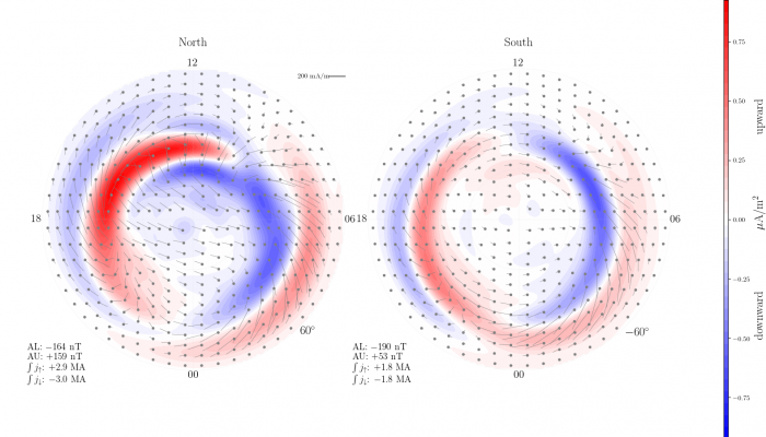
Field aligned currents (red/blue) and divergence free horizontal currents (contours) from AMPS, during the course of a day. Credit: K.M. Laundal
The AMPS model describes the average ionospheric magnetic field and current system for a given solar wind speed, interplanetary magnetic field vector, orientation of the Earth’s magnetic dipole axis, and the value of a solar flux index (F10.7). The model is empirical, which means that it is derived from measurements. We use measurements of the magnetic field, from the CHAMP and Swarm satellites, in low Earth orbit. For each measurement, model estimates of Earth’s own magnetic field, and the magnetic field associated with large-scale magnetospheric currents, have been subtracted. The remaining magnetic field is assumed to be related to ionospheric currents. Millions of measured magnetic field vectors are used to fit several thousand unknown parameters in an intricate mathematical function that describes the ionospheric magnetic field at any point in time and space. Electric currents are calculated from the magnetic field.
Model values of AMPS magnetic fields and currents can be calculated with the Python library pyAMPS, which is located here: https://github.com/klaundal/pyAMPS (documentation here: http://pyamps.readthedocs.io/).
This is not the first empirical model of ionospheric currents and magnetic fields, but there are a couple of important characteristics that sets the AMPS model apart from others: First, we have corrected for variations in Earth’s own magnetic field, which strongly distorts the ionospheric currents. This allows us to make precise comparisons between hemispheres. We have not imposed any symmetries between hemispheres; for example seasonal variations are not necessarily the same in the north and south in the AMPS model. Finally, this is the first empirical model to describe the full ionospheric current system, and not only the field-aligned part or the parts which circulates horizontally. This allows us to calculate full horizontal ionospheric current vectors without any assumptions about conductivity.
These unique features are made possible by the dataset provided by the CHAMP and Swarm missions, of very accurate magnetic field measurements from low orbit. The CHAMP satellite reentered Earth’s atmosphere in 2010, after 10 years of operation. In 2013, ESA’s Swarm satellites were launched, three satellites that carry even more precise magnetometers than CHAMP. So far, two of the Swarm satellites have flown side-by-side, near 450 km altitude, while the third satellite is a little higher. Swarm is expected to stay in space for many years, and we plan to release updated versions of the AMPS model as the data set grows. The production and publication of the AMPS model is supported by ESA through Swarm DISC.
A paper describing the model has been published in Journal of Geophysical Research – Space Physics: https://agupubs.onlinelibrary.wiley.com/doi/abs/10.1029/2018JA025387 (open access)
For more background on the technique, see an earlier paper in a special Swarm issue of Earth, Planets, and Space:
https://earth-planets-space.springeropen.com/articles/10.1186/s40623-016-0518-x (open access)