Ambient seismic noise and the quest for groundwater

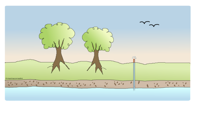
Groundwater is water stored within permeable geological formations, and nearly a third of Earth’s freshwater supply comes from this source (a). In Africa, the overwhelming majority of distributable freshwater is contained in groundwater, and in the EU, 75% of the population relies on groundwater (b).

This dependence on groundwater is steadily rising. As humanity as a whole, figures out how to adapt to the impacts of climate change and population growth on water stress, scientists have projected a 20 – 30% increase in global demand of water by 2050 (c). It follows that for sustainable water supply management, a detailed understanding of groundwater dynamics is crucial.

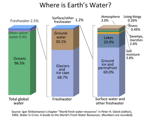
Source: Igor Shiklomanov’s chapter “world fresh resources” In Peter H.Gleick (editor) 1993, water in Crisis: A Guide to the World’s Freshwater Resources. (Numbers are rounded). Caption adapted from (a).

To study groundwater, we have several geophysical tools at our disposal: geoelectric, electromagnetic, seismic methods, and more. In the context of seismology, ambient seismic noise, in particular, is sensitive to little changes in seismic propagation velocity within a medium. And what does this velocity tell us? Seismic velocity is a seismic property of a medium, which can offer a good picture of how quickly groundwater is replenished from percolating surface water or rainfall. The main idea is that the greater the water saturation in the pores, the lower the seismic velocity (d). But how do we get from point A to point B? I’ll give a brief overview of how this works.

First, it’s worth noting that the term ‘seismic noise’ is generally used in seismology in an intuitive way. Seismic noise is the part of seismic data that is generated from unplanned sources. It is unwanted and often cannot be used to image the subsurface – often, but not always. Ambient seismic noise, in particular, is the weak, low-frequency seismic signal originating from randomly distributed sources (e). These sources may be ocean waves, human activity and even wind (f).

Next, let’s picture two seismic stations, each one comprising a seismic receiver, and let’s imagine that over a period of time, say 12 months, both of these receivers have passively been recording ‘microseismic’ signal – that is, ambient seismic noise and signal generated by mini-earthquakes. Cross-correlation is a process that quantifies the similarity between two signals, and several studies have shown that cross-correlation of the two seismic noise series collected at our stations will yield a third, more interesting signal. This new signal conveniently represents the response that would be recorded at one receiver if the other receiver were instead an active seismic source (such as a sledgehammer being slammed on a metal plate, or vibroseis, a machine that injects controlled vibrations into the ground) (g). Essentially, this new signal, the so-called ‘noise cross-correlation function’ (NCF), contains information on the earth structure between the receiver pair. In subsequent calculations, we would tend to focus more on the later parts of this NCF, the coda, because it’s more sensitive to changes in seismic properties of the earth (d)(f)(g).

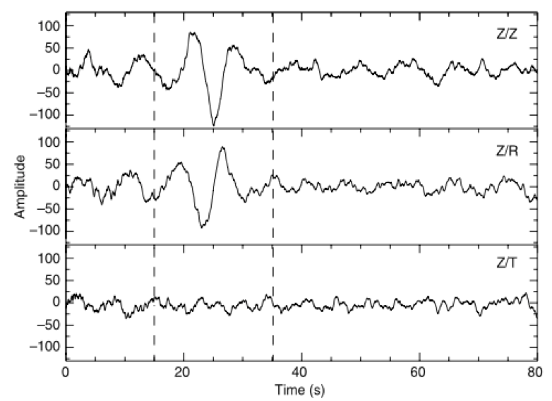
Stacked correlation functions computed from vertical component records at station PLIG and vertical (Z), radial (R), and transverse (T) component records at station YAIG. Because the individual cross-correlations were normalized before stack, the amplitudes are arbitrary. Figure and caption adapted from (g).

So how does this NCF lead us to the seismic velocity of the medium? The idea is that given our receiver pair, we could generate two NCFs, one each for two consecutive years: an NCF centered at Year 1 and the other at Year 2. Broadly speaking, we would be able to measure the time shift (dt/t) between the two different NCFs by comparing how signal in the coda shifts in time from Year 1 to Year 2 (d). dt/t can then be used to calculate the change in seismic velocity, dv/v, which in turn allows us to compute the change in groundwater level (or change in water saturation), dh, from Year 1 to Year 2. Clements and Denolle (f) present the following relationships, assuming homogenous velocity changes throughout the medium:

where β is an empirical calibration factor. The resolution can be improved by stacking NCFs, and with more than one receiver pair, we could calculate changes in groundwater volume, dV.

In the study of groundwater, one benefit of ambient seismic noise as a complement to wells is given by the fact that seismic waves scatter in the earth and thus can give insight into more minute changes in geology. This means that seismic imaging provides a more robust model of the subsurface when compared to models calculated only from individual water-wells (f). Furthermore, passive acquisition of seismic data (continuous recording of microseismic signal) is far cheaper than acquisition done by active sources, such as vibroseis. This, in turn, implies that communities with limited financial resources could conduct affordable and exciting studies in groundwater and contribute to the future of water management too.

This post was written by Aramide Moronfoye
with revisions from Michaela Wenner and Janneke de Laat

________________________________________________
References:

(a) https://www.un-igrac.org/regions/europe

(b) MacDonald, A.M, H. C. Bonsor, B. E. O. Dochartaigh and R. G. Taylor (2012),  Quantitative maps of groundwater resources in Africa, Environmental Research Letters, doi:10.1088/1748-9326/7/2/024009 (https://iopscience.iop.org/article/10.1088/1748-9326/7/2/024009)

(c) Boretti, A.  and L. Rosa (2019), Reassessing the projections of the World Water Development Report, Nature Partner Journals – Clean Water 15. (Reassessing the projections of the World Water Development Report)

(d) Fores, B., C. Champollion, G. Mainsant, J. Albaric, and A. Fort (2018), Monitoring Saturation Changes with Ambient Seismic Noise and Gravimetry in a Karst Environment, Vadose Zone J. 17:170163. doi:10.2136/vzj2017.09.0163. (https://acsess.onlinelibrary.wiley.com/doi/full/10.2136/vzj2017.09.0163)

(e) Yang, Y., and M. H. Ritzwoller (2008), Characteristics of ambient seismic noise as a source for surface wave tomography, Geochem. Geophys. Geosyst., 9, Q02008, doi:10.1029/2007GC001814 (https://agupubs.onlinelibrary.wiley.com/doi/full/10.1029/2007GC001814)

(f) Clements, T., & Denolle, M. A. (2018). Tracking groundwater levels using the ambient seismic field. Geophysical Research Letters, 45. https://doi.org/10.1029/2018GL077706 (https://agupubs.onlinelibrary.wiley.com/doi/abs/10.1029/2018GL077706)

(g) Campillo, M. and A. Paul (2003), Range Correlations in the Diffuse Seismic Coda, Science, vol. 299. (https://science.sciencemag.org/content/299/5606/547/tab-figures-data)