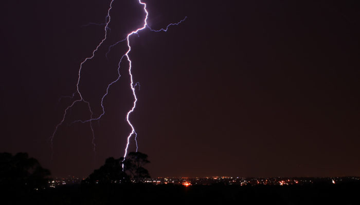
The last three decades were the warmest in the history of meteorological observations in Europe. Temperature rise is accompanied by an increase in the frequency and magnitude of extreme weather and climatic events, which are the main risks for population and environment associated with modern climate change. An important class of such phenomena includes severe rainfall, tornadoes, squalls, and thunderstorms. Given that extreme weather is expected to be the “new norm” in our rapidly changing climate, developing a forecast capability for extremes may end up becoming part of the standard prediction products that can help safeguard critical infrastructure and human lives.
In my home country, Russia, extreme weather events over the past 10 years have led to economic damage of several tens of billions of rubles (~ 1 billion Euros in today’s rates) and the death of several hundred people (e.g. heavy rainfall and floods caused by them in Krymsk in 2012 and far East in 2013 and 2016, air tornadoes in Blagoveshchensk in 2011, powerful squalls in the north of the European territory of Russia in 2010, etc.). I took some pictures of heavy thunderstorm and rain occurring in Moscow on June 14, 2016, where you can see some damages of infrastructure. (Fig. 1).
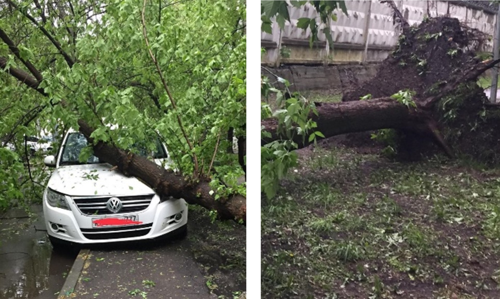
Fig. 1 Damages from severe thunderstorm in Moscow (June 14, 2016). Image credit: Inna Gubenko.
It is well known that thunderstorms are generated by cumulonimbus clouds (Fig. 2). Robust lightning prediction requires forecasting the clouds producing them. The main problem for a high-quality forecast of extreme weather phenomena is the poor understanding of specific mechanisms that determine the formation and variability of thunderstorm clouds. The reason for that is quite simple: there are very few observational data on particles in thunderclouds. Because the physical processes in a cloud are not fully described, their computer simulation is very uncertain. Despite the challenges in describing the microphysics of clouds, the importance and demand for dangerous phenomena forecasting has motivated the development of mathematical models describing the interactions of cloud particles that generate lightning. Now, let us say we have predicted the lightning – then the forecast must be verified by observed thunderstorms. However, synoptic standard observation data are sampled only every three hours, and the network of weather stations is extremely heterogeneous and sparse. This data is simply insufficient for evaluating short-term and local phenomena like thunderstorms, and further hinders improved forecasts.
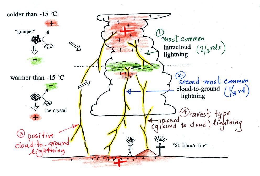
Fig. 2 Electrical structure of a Cumulonimbus cloud [3].
How is lightning formed? Let us get back again to the electrical structure of the Cumulonimbus cloud (Fig. 2). There are several types of cloud particles: graupel, ice crystals and snow. Collisions between these particles produce the electrical charge needed for lightning. When temperature is below -15° C (above the green dotted line in the Fig. 1), graupel becomes negatively charged after colliding with a snow crystal. The snow crystal is positively charged and is carried up toward the top of the cloud by the updraft winds. At temperatures between 0 and -15° C, the polarities are reversed[1]. A large volume of positive charge builds up in the top of the thunderstorm. A layer of negative charge accumulates in the middle of the cloud. Some smaller volumes of positive charge are found below the layer of negative charge. Positive charge also builds up in the ground under the thunderstorm (it is drawn there by the large layer of negative charge in the cloud). When the electrical attractive forces between these charge centers get high enough, lightning occurs. Most lightning stays inside the cloud and travels between the main positive charge center near the top of the cloud and a large layer of negative charge in the middle of the cloud; this is intracloud lightning (2/3 of all strokes). About 1/3 of all lightning flashes strike the ground. These are called cloud-to-ground discharges.[2][3] This conceptual model is the physical basis for are mathematical models for the electrical processes in convective clouds. These types of models are called electrification models. One of them is developed in the Laboratory of Atmospheric process modelling in NSI of RAS, Moscow.
I will show some results of a case study. A convective event was observed over the European part of Russia (Smolensk, Moscow, Vladimir and Nizhny Novgorod region) between 13.07.2016 and 14.07.2016. The passage of a convective storm was accompanied by a number of dangerous weather events: intensive lightning activity, rain, hail, wind squalls, and a tornado that caused human injuries, destroyed infrastructure and led to serious economic losses.[4] This weather was associated with a mesoscale convective complex (MCC) forming over border of Belarus and Smolensk region of Russia since 15:00 UTC13.07.2016. According to a radar data passage, the MCC over the Moscow region started at 18:30 UTC and was moving from North-West to East till 22:00 UTC. You can see an example of observational maps in Fig. 3 with convective (severe thunderstorm activity anomalies and hail – Fig.4) and stratiform areas with intensive cumulous precipitation[5]. After 00:00 UTC 14.07.2016, the MCC started to dissipate over Vladimir and Nizhniy Novgorod regions. The maps are colored with the type of natural hazard occurring. The goal for the future is to predict such maps.
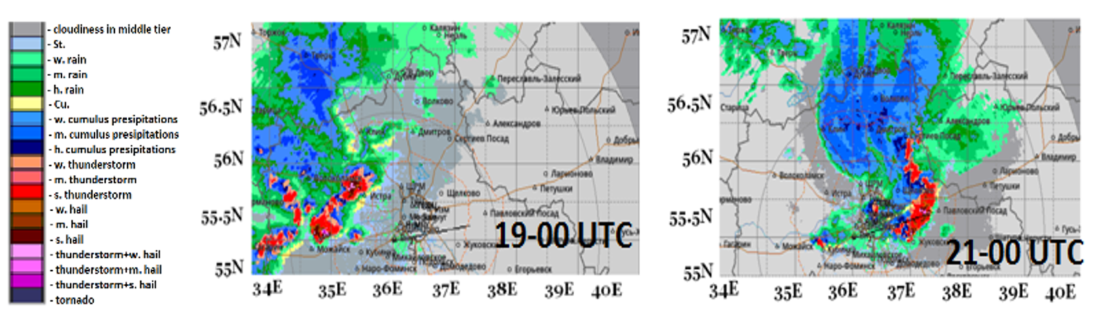
Fig. 3. Passage of a mesoscale convective complex over Moscow region, 13.07.2016. DMRL-S radar maps.
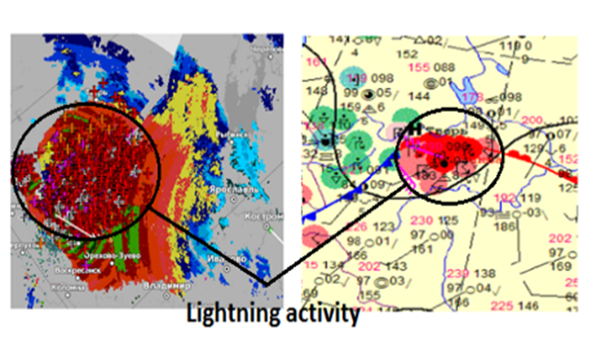
Fig. 4. Intensive lightning activity areas over Moscow region (21:00 UTC, 13.07.2016). Thunderstorm detectors and synoptic maps. Image credit: http://www.meteoinfo.ru/news/1-2009-10-01-09-03-06/12903-14072016-. Color coding same as in Fig. 4.
How well does the model predict the event shown in Fig. 3 and Fig. 4? Quite well actually, which is remarkable given the complexity and uncertainty in predicting these phenomena! Fig. 5 shows forecasting maps of simulated electric field potential difference in a layer of 0-8 km (MV) obtained by the WRF-ARW model coupled with the cumulonimbus electrification model. If we compare the radar maps (observational data, Fig. 3 and 4) and electric field maps (forecast data, fig. 5), we can see that hazardous weather events can be predicted using calculated values of the potential difference in the atmosphere. This forecast skill is considerably better than prior methods that were based on synoptic maps or statistical indices[4] and points to the power enabled by explicit, physically-based modeling of these cloud systems.[6]
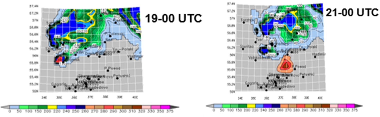
Fig. 5. Simulated electric field potential difference (MV) of mesoscale convective complex. Moscow region, 18:30-22:00 UTC, 13.07.2016. Areas where electric field potential difference exceed 260 MV indicate on thunderstorm cells (red color). Forecast maps are consistent with observational data (Fig. 3, 4).
According to these early but very promising results, this proposed approach of explicit electric field modeling is applicable to short-term forecasting of intense convection and tracking of isolated storms, convective cells and mesoscale convective complexes. Obtained varying values of the electric field could help to identify the diversity of hazardous weather phenomena associated with convection. This means, at some point we may be able to forecast severe thunderstorms. Hopefully this short time forecasting service may very soon be available on phone apps. Then you will be able to get a precise natural hazard alert in your phone weather app, so you can protect yourself in time.
Edited by Eva Pfannerstill, Mengze Li and Athanasios Nenes.
 Inna Gubenko is a Researcher, Ph. D. at the Laboratory of Atmospheric Processes Modelling in Nuclear Safety Institute of the Russian Academy of Sciences, Moscow. She focuses on mathematical modelling of convective natural hazards forecast, and thunderstorms in particular.
[1] -15° C is an empirically (laboratory) obtained temperature when cloud particles change their charge polarity. This is the so-called reverse temperature.
[2] Mansell et al. (2005) J. Geophys. Res. Atmospheres, 110, 12-20.
[3] http://www.atmo.arizona.edu/students/courselinks/fall12/atmo170a1s1/lecture_notes/nov26cmplt.html
[4] Inna Gubenko and Konstantin Rubinstein. An explicit method of mesoscale convective storm prediction for Central region of Russia. EMS Annual Meeting Abstracts. Vol. 14, EMS2017-13, 2017.
[5] http://www.meteoinfo.ru/news/1-2009-10-01-09-03-06/12903-14072016-.
[6] Previously, two methods were used for the forecasting of such phenomena. The first one is the synoptic method (analysis of synoptic maps). The second approach is based on specialized indices, taking into account only temperature, humidity and wind. Both of these two methods predict indirect signs of cloudiness. Consequently, the forecast of hazards caused by cumulus clouds by these older methods is less accurate than with electric field potential difference forecast.


Berkeley
It would be really nice if we can get to the point where we actually build phone apps that will accurately alert people against hazardous weather conditions. It’d pretty much save lives.