GeoSphere

The Most Epic Unboxing Ever

Matt Herod February 18, 2014

There is a strange phenomenon on the internet called unboxing. Unboxing is when a person receives a new package of something and takes a video or pictures of the process of opening it for the first time and posts it online. Mostly, from what I can see, people “unbox” electronics or hockey cards or things of that nature. However, what I have today could be called the granddaddy of all unboxings; I have a series of photos of the unboxing and, initial stages of set-up of the University of Ottawa’s new, 3 million volt, accelerator mass spectrometer (AMS), which cost 5 million dollars. This takes opening your new laptop or that Sidney Crosby rookie card to a whole new level!!! The AMS will be housed in uOttawa’s new Advanced Research Complex.

The accelerator portion in its shipping container being transferred into our new building. (Photo: Dr. Liam Kieser)

Easy does it. Now pivot!!! (Photo: Dr. Liam Kieser

Since I am showing pictures of this incredible piece of equipment being installed I’ll explain a bit about what it is an how it is used as well. I use the AMS in my own work to analyze iodine-129, chlorine-36 and once or twice carbon-14. In short, tools that can be used for groundwater dating. However, the AMS is capable of analyzing for a huge range of isotopes and this allows its use a wide variety of disciplines from health science to homeland security.

The AMS works on the same principles and a regular mass spectrometer, but it has a few key differences that make it extremely powerful.

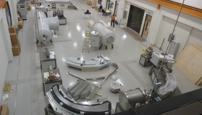
Lots of boxes to open. (Photo: Dr. Liam Kieser)

Once the boxes have been unloaded the building begins. It is like building an IKEA desk, but somehow more… (Photo: Dr. Liam Kieser)

The process of AMS analysis begins with the preparation of the samples, which involves large amounts of lab time in extremely clean conditions. Contamination of samples with unwanted isotopes is a real problem in AMS so great care has to be taken to prepare good samples. The sample is then mixed with niobium powder and pressed into a steel cartridge. The cartridge then gets loaded into the ion source where cesium ions get fired at the sample like shooting a gun. The Cs ions physically break bits of the sample off the cartridge and these get negatively ionized and accelerated out of the ion source towards the first magnet.

Xiao-lei carefully taking the glass rings that are in the accelerator. These are to kill any free electrons that could escape from the stripper canal as well as keep the ions on a stable flight path. X-rays charged to 3 million volts are very bad! (Photo: Dr. Liam Kieser)

The glass rings all put together with the stripper canal in the centre. The stripper canal is where electron get stripped off the negative ions turning them into positive ions as well as keeping the ions on a straight and even flight path. (Photo: Dr. Liam Kieser)

This is what the ion source looks like. Up to 200 samples sit in the big wheel waiting their turn. The AMS control room is those windows in the background.

Our fancy new SO-110 ion source. (Photo: Matt Herod)

Once the samples leave the ion source they are accelerated to the first bending magnet which can bend an incredible range of masses. From tritium to plutonium tri-fluoride.

The first magnet looking towards the accelerator. (Photo: Matt Herod)

The next step is firing the ion into the particle accelerator that carries a charge of 3 million volts! Inside the accelerator is a passage called a stripper canal that pulls electrons off the ions turning them from negative into positive ions. The reason for this is that this allows us to get rid of interferences that normal mass spectrometers face. For example, chlorine-36 has an interference with sulphur-36 making it impossible to analyse using normal mass specs. Actually, our AMS has another modification that makes 36Cl analysis possible on a 3MV machine, which is generally considered too small for this isotope. Usually, 36Cl needs a much larger accelerator however, our isobar separator for anions (ISA) allows this. Once the ion leaves the stripper canal it is accelerated at very great speed into the next magnet.

Dunh, dunh, dunh. This is the A in AMS! (Photo: Matt Herod)

This is the biggest magnet I have ever seen!! It is over 3m long and weighs 18 tonnes! This is why the room needs an overhead crane. (Photo: Matt Herod)

Once the ions are redirected and isotopes are further separated by the magnet they are ready to be analyzed in either the Faraday cups for the common isotopes or the gas ionization detector for rare isotopes.

Me, touching the Faraday cups. (Photo: Laurianne Bouchard)

The gas ionization detector. This bad boy literally counts atoms as they come around yet another magnet and through a silicon nitride window. Once they enter the detector which is filled with gas they ionize it which leads to pulses of electricity that are counted. This is the end of the AMS!!! (Photo: Matt Herod)

Once the atoms are counted in the gas ionization detector their trip around the AMS is over! It is quite a journey and full of positives and negatives (haha, a little pun there). Seriously, though this gigantic instrument is used to quantify the smallest of small quantities and can very literally count atoms. The AMS has a massive number of possible uses and I’ll likely be posting about these as this new facility starts to ramp up in the next few months. In addition to the AMS we also have an SEM, microprobe, stable isotope equipment, two noble gas mass spectrometers, ICP-MS, LA-ICP-MS, ICP-AES and a host of other MS’s as well. There will be very few types of isotopes that we cannot analyze for and this facility will be one of the best in the world for this type of geological research. Stay tuned for further developments as we start to move in soon!

Cheers,

Matt

Some 2014 Ph.D Goal Setting

Matt Herod January 16, 2014

For my first post of the new year I thought it might be a good idea to make some resolutions, especially since everyone else is doing it. Part of doing graduate work is setting goals, ignoring those goals until the week before, and then working 22 hour days to achieve them. Ian, (my supervisor), if you’re reading this I swear that is just a joke!

Source – “Piled Higher and Deeper” by Jorge Cham. www.phdcomics.com

In all seriousness though I am hoping that 2014 will be a big year for me. My ultimate goal is to have hopefully defended by this time next year or at the very least submitted my thesis. Of course, I am falling into the obvious trap pictured below by publicly announcing my intent to finish within a year.

Source – “Piled Higher and Deeper” by Jorge Cham. www.phdcomics.com

However, I think that if I set reasonable goals and work really damn hard I can get this thesis done. Hopefully, no major issues occur in the lab or elsewhere that delay things. The easiest way to accomplish this Herculean task is to break it down into somewhat more bite-sized chunks and tackle those one at a time. Trying to think of this as a whole will not help me accomplish anything. Luckily for me uOttawa accepts thesis’s? theses? that are composed of a collection of separate articles, which is the format that I’ll be using.

2014 Goals

– Finish paper on combustion technique – this is nearly done, just have to respond to the journal reviewer comments.

– Continue writing Fukushima paper. Getting there…..this one is not writing itself at the moment, but I am making slow progress every day. If you were at Goldschmidt 2013 you heard this talk.

– Finish all lab work related to iodine and 129I transfer in the Wolf Creek watershed and synthesize data – this is also nearly done, just a few more samples to run on the AMS. Of course the data synthesis and some statistical analysis will take some time.

– Write paper on Wolf creek watershed, make figures, etc.

– Data synthesis and writing of large scale Yukon watersheds project. Got a paper to write here now that I have all the data. Of course there is lots of work to do still on figure making and data analysis as well.

– Learn about noble gas extraction and fissionogenic xenon isotopes…also learn more about stats.

– Start combustion extractions of iodine in Bruce deep geologic repository site core and analyze on AMS and ICP-MS.

– Go to England and analyze xenon isotopes in Lancaster???? Not sure if this is happening yet. Fingers crossed!

– Synthesise data and write paper on fissionogenic isotopes in ancient groundwater.

– Go to a conference, be it AMS13 in France, GSA in Vancouver, etc….or maybe go to two.

– Get some writing done at the cottage this summer!!!! Very important.

– Staple all this crap together and turn it in.

– Defend! Oh god, I hope this one happens in 2014!

I am flip-flopping between the last two panels at the moment! (Source) – “Piled Higher and Deeper” by Jorge Cham. www.phdcomics.com

Wish me luck, oh yeah, I have to do some blogging here and there as well. On that vein, I would love to have a few more guest posts, since as you can see I am going to be busy this coming year. So if you read this, and are interested in sharing your research, please contact me in the comments or on twitter and we can arrange something.

Matt

Guest Post: Hilary Dugan – Ice as a platform for understanding lake ecosystems

Matt Herod January 13, 2014

Today we have a new guest post written by current PhD candidate and Antarctic researcher on her very fascinating field work. Actually, she wrote this post while at McMurdo station. Hilary and I have known each other since our time at Queens University in Kingston, when she was one of my TA’s and was doing her masters. For more info about her work see the bio at the end of the post at check out her own excellent blog.

In Antarctica, there is a small swath of land hidden by the Transantarctic Mountains that is too dry and sheltered to be overridden by the ice sheets that cover over 99% of the continent. In these barren valleys, life is at the edge of existence and sustained by pulses of meltwater that form when summer temperatures finally break the freezing point. The only refuges of perennial water in this habitat are the large lakes that occupy the topographic depressions in the valley bottoms. The lakes themselves are hidden beneath permanent ice covers of 4 m, but reach depths of 20 to 75 m, and temperatures of -13 degC to +25 degC. As a colleague remarked, “This system of valleys is one of the coldest and driest places in the world and has more in common with Mars than it does with your backyard”.

Don Jon Pond (the saltiest body of water on Earth) in Wright Valley, Antarctica

The McMurdo Dry Valleys is also one of the only places in the world with year-round lake ice, which is partly why I spend a few months of the year hidden beneath a giant red parka. Imagine studying the atmosphere without solid ground. Where would we build telescopes, satellite dishes, or research stations? In oceanography and limnology, this is a fundamental roadblock in the collection of long-term data, and is amplified in remote and deep environments where ships or divers can be logistically impossible to send.

Downloading datalogger at Lake Fryxell, Antarctica

Luckily for polar researchers (and everyone else *), the solidification of water into ice happens at relatively warm temperatures (0 degC for freshwater, -1.9 degC for ocean water) and floats, thereby providing a frozen platform to access the hidden ecosystem beneath. In most temperate environments, this advantage is limited to a few winter months, and in the shoulder seasons, ice is viewed as a destructive force capable of destroying or dragging around all but the sturdiest of instrumentation. The result is most high-resolution lake data is acquired from spring to fall before buoys are pulled for the winter. Ice is both a boon and a barrier for limnology.

Lake Bonney, Antarctica. Blood Falls can be seen at the edge of Taylor Glacier in the lower right hand corner.

The permanent ice covers in the Dry Valleys allow us to moor instrumentation beneath the ice cover year round, which is a rarity in limnology. Below 4 m of ice, we record physical parameters, such as ice thickness, underwater radiation, ice ablation, and lake level. Our research is primarily focused in Taylor Valley, which has been an US National Science Foundation LTER (Long Term Ecological Research) site for the past twenty years. Three large closed-basin lakes span a range of physical conditions, and represent some of the saltiest and coldest bodies of water on Earth. Because the lakes harbor liquid water year-round, the lakes may be the microbial Amazon of the Dry Valleys; even though the ecosystem is made up of a simple trophic structure. This simplicity allows biological processes and interactions to be more easily studied than in more biologically complex habitats.

Surface dataloggers at Lake Hoare, Antarctica

This long-term data allows us to track the habitability of lakes, and general hydrology of the watershed. For instance, the last decade has seen a tremendous rise in lake levels, and therefore a positive water balance in the Valleys. This has come without a concomitant increase in temperature, and researchers are currently investigating the trigger for meltwater production in this water-starved environment.

In our goal of year-round monitoring, one major hurdle is that biologic sampling is only conducted during the summer, when the temperatures are reasonable enough for personnel to be in the field. Therefore, any assumptions of microbial activity during the polar winter have been extrapolated from data procured mainly from Oct to Jan (one very cold season stretched until April).

This field season, our goal was to fill in the missing months, and for the first time understand ecosystem functioning during a period of total darkness; a subject extremely valuable to those studying the habitability of environments outside our planet. Instead of over-wintering in Antarctica (we’re not that crazy), we moored three large automated instruments in Lake Bonney: a water sampler, a phytoplankton sampler, and a profiling CTD equipped with a fluorometer and CO2, dissolved oxygen, and PAR sensors. These instruments will be collecting data and samples until our return in Nov. 2014.

Deployment of an automated phytoplankton sampler in Lake Bonney, Antarctica.
Pictured: Luke Winslow (University of Wisconsin, Madison), Kyle Cronin and Dr. Peter Doran (University of Illinois, Chicago)

This winter it will be 40 years since the New Zealand program’s last overwinter campaign in Wright Valley. While they braved complete darkness and colder temperatures than most of us have ever experienced in the pursuit of meteorological measurements, I will be nestled warmly in Chicago knowing that somewhere far away a CTD will be capturing the first winter data from one of the most unique lakes on the planet.

As otherworldly as Antarctica may seem, the life that exists in this frozen corner of the Earth demonstrates the incredible adaptation of organisms to surrounding environments, and is likely the closet planetary analogue to any life that may exist on other icy planets in our solar system. Perhaps one day in the future, some young scientist will be making the same comments about their research beneath the icy shell of Europa.

* – If ice was denser than water (like the solid form of most liquids) the ocean would freeze from the bottom up, drastically changing ocean circulation and climate.

I am a PhD candidate at the University of Illinois at Chicago, working with Dr. Peter Doran in the Department of Earth and Environmental Sciences. My current research focus is on Antarctic limnology, with the overarching hypothesis that small variations in climatic conditions can result in extreme hydrologic shifts. I am actively involved in three Antarctic projects: one which examines the hydrology and microbiology of a unique lake with a 27+ m ice cover, a second which uses geophysical techniques to map subsurface brines beneath lakes, and a third which focuses on long term limnological changes as part of the McMurdo Dry Valleys Long Term Ecological Research (LTER) program.

One of my responsibilities is to maintain long-term data sets associated with the physical properties of the McMurdo LTER lakes. This includes field-based implementation of lake stations, upkeep of instrumentation, data compilation and management, and ultimately, analysis of the data sets. I regularly employ analytical tools, such as R, Matlab, and ArcGIS, to both to post-process data and explore spatial imagery.

For more information, feel free to visit: https://sites.google.com/site/hilarydugan/
Or check out my field blog at: http://b511m.wordpress.com/

Reading Past Sea Ice Coverage from strange red blobs!

Matt Herod December 13, 2013

Sea ice is an interesting phenomenon, especially to a Canadian. The question around this time of year that always arises in the news is will this be a big sea ice year, will we set a new record low, high (haha) or will it be just average? This is a question that gets a lot of study and media attention. People run countless statistical models to predict sea ice conditions and try to predict the past and future conditions based on these annual observations. It is a nerdy admission but there are two things I follow religiously on the web: sea ice coverage and NHL standings (Go Leafs!!)….ah, who I am kidding, it is mostly about sea ice. So, you can imagine my interest the other day when I came across an article on the CBC about a new proxy for measuring past sea ice coverage. Even stranger was that fact that this new proxy was corralline algae, which I had been looking at in thin section earlier that day in my role as a carbonate sedimentology TA. It is a strange ol’ world.

2005 NASA Sea Ice extent Imagery. (Source) – Wikimedia Commons – NASA

Anyway, this new paper entitled “Arctic sea-ice decline archived by multicentury annual resolution record from crustose corraline algal proxy” recently appeared in PNAS. In this study the authors used corralline algae as a new proxy to estimate sea ice coverage in the Arctic. The question that these authors sought to answer using corraline algae as a proxy was: can we calculate past sea ice coverage and can we then use the larger knowledge base we now have about past sea ice to apply that to predicting future sea ice conditions given at current models are not very reliable at predicting future sea ice coverage?

First, lets look at this corraline algae proxy. Corraline algae is a type of red algae that have been around since Cretaceous. As the name suggests they tend to be red in colour and often grow in coral reefs. According to Wikipedia appear as “pink to pinkish-grey patches, splashed as though by a mad painter over rock surfaces”. (How poetic eh?). Anyway, they are widely distributed globally and occur in all the world’s oceans up to the maximum depth light can penetrate as they are photosynthetic and their growth depends on light and temperature. The species of corraline algae used in this study was Clathromorphum compactum, which forms a new layer ever year, much like a tree forms rings. Clathromorphum is an encrusting variety of red algae that grows on rocky substrates year after year essentailly in perpetuity as the only thing that can prevent it from adding another high Mg calcite later is if something actually breaks it apart or eats it. The authors found samples of Clathromorphum up to 646 years old!

Photo of coralline algae – Wikimedia Commons – Author: Derek Keats

The way a proxy works is that a certain feature of the sample, such as its chemistry or growth ring width, can be used to tell us about conditions that were responsible for chemical changes in the sample or the size of its growth rings. It is even better if the sample can be used to represent large time periods. Therefore a sample of 646 year corralline algae has the potential to be used as a proxy if its chemical or growth features are caused by a change in living conditions. As it happens the growth of corralline algae is directly related to amount of sun in receives. For example, if it is very sunny the algae will have larger growth rings, if it is not sunny the algae will have very small growth rings. Furthermore, when the algae is growing it preserves the Mg/Ca ratio of the seawater it is growing in inside its calcite skeleton. However, if the algae is not growing the recording of Mg/Ca ratios stops. So, if there is no sea ice the algae makes thicker growth rings and has a high Mg/Ca ratio, when there is sea ice covering the area the algae is growing in the growth rings are small and the Mg/Ca ratios are low. The fact that coralline algae has two proxies that can tell us about sea ice conditions makes it an excellent tool for looking into the past to see ice coverage. It is a great double whammy!!

Fig. S2. Analytical reproducibility. Annual cycles of Mg/Ca ratios measured by electron microprobe (A) on two parallel transects along main axis of growth on uppermost 5 mm of sample Ki2 (B). Microscope image of polished sample shows ∼80 annual growth increments. Cycle shapes in A are characteristic of break in growth during sea-ice season, with narrow downward pointing peak. Summer portions of cycles instead are smooth, reflecting summer light and temperature cycle patterns following spring breakup of sea ice. Note similarity of winter Mg/Ca ratios reflecting constant seawater temperature under sea ice. Sample spacing, 15 μm (average annual growth of Ki2 = 172 μm) results in average resolution of ∼11.5 samples per year. Mg/Ca ratios are based on atom percent of Mg and Ca. Photo and caption used in accordance with PNAS guidelines for educational purposes only.

So, based on the fact that the size of the growth rings and Mg/Ca ratios in the growth rings of Clathromorphum tell us about sea ice coverage the authors set out to sample Clathromorphum from a variety of locations around Northern Canada. What they found is pictured in the figure below, but I’ll cover the highlights.

1. The record of sea ice coverage obtained from the coralline algae proxy agrees well with known sea ice coverage data from the 1970’s onwards.

2. The algal proxy shows that sea ice coverage has been declining steadily for the past 150 years, the latter part of which agrees with actual observations of sea ice coverage.

3. A 646 year record shows that sea ice coverage was high between 1530 and 1860, which corresponds to the Little Ice Age.

4. The results from this proxy agree well with those from other proxies such as ice cores and anthropological evidence for high sea ice coverage during the Little Ice Age.

Fig. 3. Algal proxy record (red) compared with observational (blue) and proxy (green) data (see Methods for detail on records). Gray lines represent 5-y moving average and colored lines, 15-y low-pass filtered (Savitzky–Goley) annual data. Algal proxy time series plotted on inverted scale to indicate declining ice cover. Light gray bars show periods of positive algal anomalies, reflected by negative ice anomalies in observational records, and positive δ18O ice core excursions. Linear trends for all time series are plotted from 1850 onwards. All individual algal specimens yield similar trends (Fig. S3). RC indicates position of radiocarbon analyses. Values are 2σ calibrated results (Table S1); all values fall well within age model derived from growth increment counting.

So there it is. Coralline algae is a great new proxy for sea ice coverage. I am left wondering a few things about the use of this proxy that hopefully the authors will address in future work. The foremost question in my mind is: could this be used as a proxy for sea ice coverage into the distant past? We find a lot of coralline algae in the fossil record so perhaps if the paleo-latitude was known, these preserved specimens could be used to interpret sea ice conditions thousands or even millions of year ago? What do you think? I’m not sure how well Mg/Ca ratios are preserved, but the growth rings certainly are….

Halfar J., Adey W.H., Kronz A., Hetzinger S., Edinger E. & Fitzhugh W.W. (2013). Arctic sea-ice decline archived by multicentury annual-resolution record from crustose coralline algal proxy, Proceedings of the National Academy of Sciences, 110 (49) 19737-19741. DOI: 10.1073/pnas.1313775110

The article that first called my attention to this paper.