Geochemistry

Reading Past Sea Ice Coverage from strange red blobs!

Matt Herod December 13, 2013

Sea ice is an interesting phenomenon, especially to a Canadian. The question around this time of year that always arises in the news is will this be a big sea ice year, will we set a new record low, high (haha) or will it be just average? This is a question that gets a lot of study and media attention. People run countless statistical models to predict sea ice conditions and try to predict the past and future conditions based on these annual observations. It is a nerdy admission but there are two things I follow religiously on the web: sea ice coverage and NHL standings (Go Leafs!!)….ah, who I am kidding, it is mostly about sea ice. So, you can imagine my interest the other day when I came across an article on the CBC about a new proxy for measuring past sea ice coverage. Even stranger was that fact that this new proxy was corralline algae, which I had been looking at in thin section earlier that day in my role as a carbonate sedimentology TA. It is a strange ol’ world.

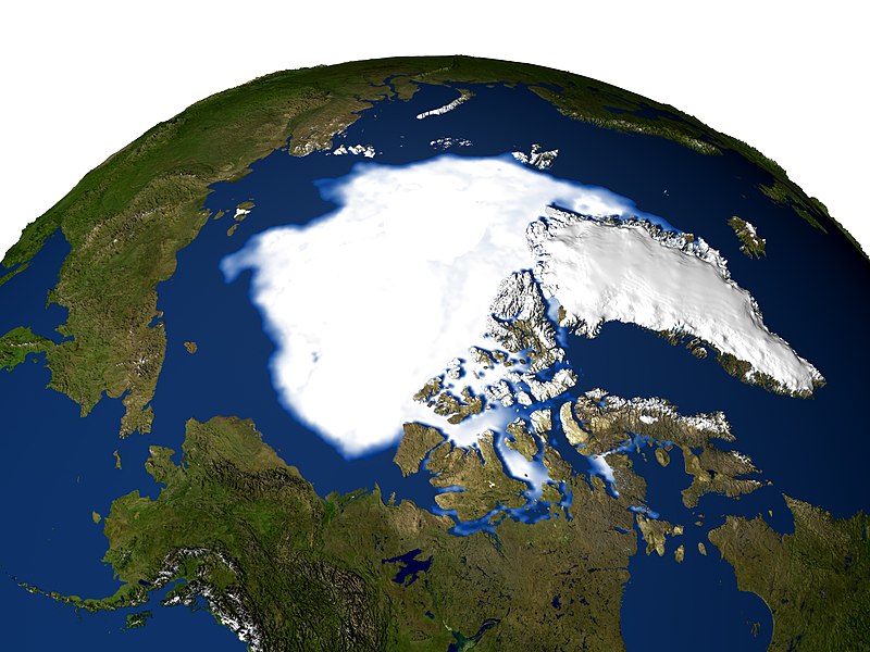
2005 NASA Sea Ice extent Imagery. (Source) – Wikimedia Commons – NASA

Anyway, this new paper entitled “Arctic sea-ice decline archived by multicentury annual resolution record from crustose corraline algal proxy” recently appeared in PNAS. In this study the authors used corralline algae as a new proxy to estimate sea ice coverage in the Arctic. The question that these authors sought to answer using corraline algae as a proxy was: can we calculate past sea ice coverage and can we then use the larger knowledge base we now have about past sea ice to apply that to predicting future sea ice conditions given at current models are not very reliable at predicting future sea ice coverage?

First, lets look at this corraline algae proxy. Corraline algae is a type of red algae that have been around since Cretaceous. As the name suggests they tend to be red in colour and often grow in coral reefs. According to Wikipedia appear as “pink to pinkish-grey patches, splashed as though by a mad painter over rock surfaces”. (How poetic eh?). Anyway, they are widely distributed globally and occur in all the world’s oceans up to the maximum depth light can penetrate as they are photosynthetic and their growth depends on light and temperature. The species of corraline algae used in this study was Clathromorphum compactum, which forms a new layer ever year, much like a tree forms rings. Clathromorphum is an encrusting variety of red algae that grows on rocky substrates year after year essentailly in perpetuity as the only thing that can prevent it from adding another high Mg calcite later is if something actually breaks it apart or eats it. The authors found samples of Clathromorphum up to 646 years old!

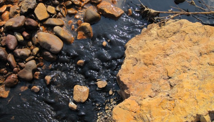
Photo of coralline algae – Wikimedia Commons – Author: Derek Keats

The way a proxy works is that a certain feature of the sample, such as its chemistry or growth ring width, can be used to tell us about conditions that were responsible for chemical changes in the sample or the size of its growth rings. It is even better if the sample can be used to represent large time periods. Therefore a sample of 646 year corralline algae has the potential to be used as a proxy if its chemical or growth features are caused by a change in living conditions. As it happens the growth of corralline algae is directly related to amount of sun in receives. For example, if it is very sunny the algae will have larger growth rings, if it is not sunny the algae will have very small growth rings. Furthermore, when the algae is growing it preserves the Mg/Ca ratio of the seawater it is growing in inside its calcite skeleton. However, if the algae is not growing the recording of Mg/Ca ratios stops. So, if there is no sea ice the algae makes thicker growth rings and has a high Mg/Ca ratio, when there is sea ice covering the area the algae is growing in the growth rings are small and the Mg/Ca ratios are low. The fact that coralline algae has two proxies that can tell us about sea ice conditions makes it an excellent tool for looking into the past to see ice coverage. It is a great double whammy!!

Fig. S2. Analytical reproducibility. Annual cycles of Mg/Ca ratios measured by electron microprobe (A) on two parallel transects along main axis of growth on uppermost 5 mm of sample Ki2 (B). Microscope image of polished sample shows ∼80 annual growth increments. Cycle shapes in A are characteristic of break in growth during sea-ice season, with narrow downward pointing peak. Summer portions of cycles instead are smooth, reflecting summer light and temperature cycle patterns following spring breakup of sea ice. Note similarity of winter Mg/Ca ratios reflecting constant seawater temperature under sea ice. Sample spacing, 15 μm (average annual growth of Ki2 = 172 μm) results in average resolution of ∼11.5 samples per year. Mg/Ca ratios are based on atom percent of Mg and Ca. Photo and caption used in accordance with PNAS guidelines for educational purposes only.

So, based on the fact that the size of the growth rings and Mg/Ca ratios in the growth rings of Clathromorphum tell us about sea ice coverage the authors set out to sample Clathromorphum from a variety of locations around Northern Canada. What they found is pictured in the figure below, but I’ll cover the highlights.

1. The record of sea ice coverage obtained from the coralline algae proxy agrees well with known sea ice coverage data from the 1970’s onwards.

2. The algal proxy shows that sea ice coverage has been declining steadily for the past 150 years, the latter part of which agrees with actual observations of sea ice coverage.

3. A 646 year record shows that sea ice coverage was high between 1530 and 1860, which corresponds to the Little Ice Age.

4. The results from this proxy agree well with those from other proxies such as ice cores and anthropological evidence for high sea ice coverage during the Little Ice Age.

Fig. 3. Algal proxy record (red) compared with observational (blue) and proxy (green) data (see Methods for detail on records). Gray lines represent 5-y moving average and colored lines, 15-y low-pass filtered (Savitzky–Goley) annual data. Algal proxy time series plotted on inverted scale to indicate declining ice cover. Light gray bars show periods of positive algal anomalies, reflected by negative ice anomalies in observational records, and positive δ18O ice core excursions. Linear trends for all time series are plotted from 1850 onwards. All individual algal specimens yield similar trends (Fig. S3). RC indicates position of radiocarbon analyses. Values are 2σ calibrated results (Table S1); all values fall well within age model derived from growth increment counting.

So there it is. Coralline algae is a great new proxy for sea ice coverage. I am left wondering a few things about the use of this proxy that hopefully the authors will address in future work. The foremost question in my mind is: could this be used as a proxy for sea ice coverage into the distant past? We find a lot of coralline algae in the fossil record so perhaps if the paleo-latitude was known, these preserved specimens could be used to interpret sea ice conditions thousands or even millions of year ago? What do you think? I’m not sure how well Mg/Ca ratios are preserved, but the growth rings certainly are….

Halfar J., Adey W.H., Kronz A., Hetzinger S., Edinger E. & Fitzhugh W.W. (2013). Arctic sea-ice decline archived by multicentury annual-resolution record from crustose coralline algal proxy, Proceedings of the National Academy of Sciences, 110 (49) 19737-19741. DOI: 10.1073/pnas.1313775110

The article that first called my attention to this paper.

New study shows nitrate leaches to groundwater for over five decades

Matt Herod November 12, 2013

A new and very interesting study just came out in the journal Proceedings of the National Academy of Sciences (PNAS) the other day titled “Long-term fate of nitrate fertilizer in agricultural soils”. This paper addresses some very interesting and extremely important questions using isotopic geochemical tools.

The question central to this paper is what happens to all of the nitrogen in the fertilizer that we spread on our crops? This question is a very popular one in the nitrate contamination field (haha, pun intended) and this paper attempts to look at the long term fate of this molecule, which is an aspect that is not very well understood. The paper looks at a field that had nitrate fertilizer labelled with the stable isotope nitrogen-15 spread over it for three decades to see what the fate of this nitrogen is? In other words, where does it go? Does it stay in the same place? Is it still available to plants or does it end up in the groundwater or surface water? In fact, the authors found that 61-65% of the applied fertilizer was used by plants, and 12-15% was still in the soil. Furthermore, 8-12% of the nitrogen added had entered the hydrosphere during the 3 decade observation period and the fertilizer remaining in the soil was still available to crops and to leak into groundwater over the upcoming fifty years.

Let’s take a quick step back though. Why is nitrogen, an element that is essential to the health of plants and one of the basic elements found throughout the the natural world being considered a contaminant? There are two main reasons that having excess nitrate, which is NO3, in the hydrosphere is a problem. The first is eutrophication. Eutrophication is a phenomenon that occurs when excessive nutrients enter a water body. The additional nutrients cause massive plant growth including algae. This leads to an occurrence called an algae bloom, pictured below, that covers the water surface, preventing other plants from photosynthesising and leading to their death. This mass die-off consumes all of the oxygen in the water body and leads to the death of the entire food web. In short nutrient overloading leads to the apocalypse.

Algae bloom in Florida. (Source)

The second reason that high levels of nitrate are a concern is because of a health problem associated with people and animals consuming excess nitrate called Methemoglobinemia, which is also known as blue baby syndrome. This disease affects the chemistry of the blood and prevents the transfer of oxygen from the blood to tissues. This occurs most often in babies under 6 months of age and can be caused by elevated nitrate levels in their drinking water. It is for this reason that the maximum allowable concentration of nitrate in most place is 10 ppm.

Ok, back to the study. So the authors found that there are three places where the added nitrate can end up over time and this finding is pictured in the graph below. What this figure is showing is that immediately after adding the fertilizer in 1983/84 the total load of N03 in the plants goes up 50% immediately, which is good for growing things. A further 30-40% is trapped in soil organic matter. The total of both these reservoirs roughly equals 100% of the expected NO3 load.

However, over time the amount in the plants slowly increases while the reservoir of labelled NO3 in the soil organic matter decreases at a much faster rate. This loss of NO3 from the SOM is being found in sampling lysimeters showing that it is leaching off the SOM and ending up in groundwater. The NO3 that is trapped in the SOM mixes with the existing nitrate that is already there and is then slowly leached over the next several decades. In fact, the authors found that 0.4% of the labelled nitrate leached per year and during the study period 8-12% of the labelled fertilizer ended up leaching off the SOM into the groundwater! This may not seem like a lot but considering the massive volume of fertilizer spread in agricultural regions each year this can add up to a huge annual influx of NO3 to the hydrosphere and have serious environmental repercussions.

Cumulative budget of 15N-labeled fertilizer nitrogen based on mass and isotope balances for plants, soil organic matter (SOM), and nitrate in lysimeter outflows for Lys S (full symbols) and Lys W (empty symbols). Image from Sebilo et.al. (2013) and used according to PNAS copyright guidelines for educational purposes only.

The next thing the authors tested, which is pictured in the figure below, was to see how far into the future the labelled fertilizer will continue to leach to the groundwater. The data points that have already been collected are pictured and a decay function, such as exponential decay, is fitted to them. As you can see the decay function fits the existing data nicely and therefore can be used to predict what could happen in the future. The graph is showing that it will take another five decades for the values 15N in the soil to return to background i.e. pre-application of the 15N labelled fertilizer levels. Basically, this means that the single application of 15N enriched fertlizer in 1981 will have an influence on soil nitrate and hence leaching for 100 or more years.

Decay functions fitted to observed δ15N values of soil organic matter from Lys S (red) and Lys W (blue). The model suggests that it will take circa 100 y to reach the background δ15N values of circa +5‰ observed before tracer application. Image from Sebilo et.al. (2013) and used according to PNAS copyright guidelines for educational purposes only.

To summarize, the study by Sebilo et.al. found that the fertilizer that gets added to fields all over the world is not immediately taken up by plants. In fact, it sits around in soil organic matter and can slowly leach into groundwater over 50 or more years! This is a major cause for concern and understanding the dynamics of nitrate in soil over long time periods will help us avoid some of the potential environmental or health problems that fertilizing could cause. Indeed, we now know that simply waiting for the nitrate we add to disappear naturally is not an option as the SOM provides a continuous source of nitrate.

Here is the link that alerted me to this article in the first place:

http://www.waterworld.com/articles/2013/10/nitrogen-fertilizer-remains-in-soils-and-leaks-towards-groundwater-for-decades-researchers-find.html

Reference:

Mathieu Sebilo, Bernhard Mayer, Bernard Nicolardot, Gilles Pinay, and André Mariotti
Long-term fate of nitrate fertilizer in agricultural soils
PNAS 2013 110: 18185-18189.

PDF: http://www.pnas.org/content/110/45/18185.full.pdf+html

Thanks for reading, especially if you read the whole thing!

Matt

AW# 60 – Radioactivity: What’s the use?

Matt Herod October 1, 2013

Cherrenekoff radiation is a pretty way to demonstrate radiation. (Photo: Matt Herod)

I am very excited to be hosting the 60th Accretionary Wedge at GeoSphere! Sorry my own contribution is so slow in coming…it has been a busy month PhD wise. In fact, I expect it will be a busy year PhD wise since I am hoping to submit in the Fall of 2014 and I have got a LOT of writing to do. Anyway, in the call for posts I said:

For this wedge the topic will be momentous discoveries in geology or its sub-disciplines that you feel have altered or shaped our understanding of how the Earth works, or opened new doors into research that had never been considered before. The discovery you choose does not have to be universally recognized as momentous but should be in your opinion. It could be something that we take for granted every day, but is in actuality part of the underpinnings of our science.

The discovery I am going to discuss is one that a wide variety of different geoscience disciplines uses every day and one that is particularly near and dear to my heart, since my PhD. is about an application of this discovery: radioactivity and radioactive isotopes. The consequences of the discovery of radioactivity have been extremely far reaching in many fields, particularly the geosciences. For this post I am not going to describe what radioactivity is, but rather some of the fantastic applications and subsequent discoveries that have hinged on the initial discovery of radioactivity and radioactive elements. There are a lot, so for the ones I don’t talk about I’d love to see comments on.

Cherrenekoff radiation is a pretty way to demonstrate radiation. (Photo: Matt Herod)

Cherenkov radiation is a pretty way to demonstrate radioactivity. (Photo: Matt Herod)

The Earth is constantly in a state of change. The process that move and shape the Earth are doing so in front of our very eyes. If only we had a means to see it happen….oh wait. Radioactive isotopes can often be used as tracers of natural processes. Sometimes the isotopes are naturally occurring and sometimes they are added through human activities. Either way, we can use them to uncover Earth’s mysteries.

The first thing that everyone thinks about when discussing application of radioisotopes in geology is radioactive dating. The basic principle of radioactive dating was discovered by Ernest Rutherford in 1905 and states that if we know the half life and the concentration of the decay product we can use that information to calculate how much of the parent isotope there was and then how old the material the daughter product was measured in is. This basic idea has spawned a wide variety of dating techniques using different isotopes with a range of half lives from very short to very, very long. Radioactive dating is the reason we know old the Earth is, when the dinosaurs lived and died, when ancient volcanoes erupted, what sort of tectonics took place on the early Earth, how long ago our ancestors lived and so much more. The problems to which radioactive dating can be applied are limited by the presence of a usable isotope rather than running out of questions. Indeed, there will always be more things to date using the wide varity of isotopes available. It is possible to date recent things using Carbon 14 or Tritium (Hydrogen), which both have fairly short half lives. The furthest back that I have seen dating methods go is for rocks from the Isua Greenstone belt, which were dated at 4.28 billion years using the samarium-neodymium isotope system (Note: This work was done by J. O’Neil a new prof at uOttawa). Either way, if it is new or old radioisotopes can date it.

Occasionally pollution can be useful. It goes without saying that pollution is bad. However, on occasion its presence can be used to solve scientific problems when nature does not provide a means to do so. One instance of this is using radioactive releases from nuclear fuel reprocessing to trace ocean currents in the North Atlantic ocean. The releases themselves are extremely low level, and are not dangerous to humans or the ecosystem in any way. However, they are easily detectable and therefore can be used. Fuel reprocessing releases a lot of iodine-129 and cesium-137, as well as some other isotopes. These isotopes are then released into the Atlantic ocean and circulate with currents. Using these isotopes to trace the depth profile of currents, where they move and how long it takes for them to circulate is a burgeoning field in oceanography research.

Not all radiotracers are pollution though. Ideally, we can use naturally produced radiotracers to tell us about the environment. For example, contaminated places aside, radon is produced by the decay of naturally occurring uranium-238. It can then be incorporated into groundwater or pass through the soil as a gas. One immediately obvious use of radon is in uranium exploration. If there is a higher concentration of uranium in the rocks more radon will be produced. Therefore, if soil gas sampling for uranium exploration finds elevated radon that could be an indication of a possible economic uranium enrichment. Another way of using radon is something that I have some personal experience with: tracing groundwater discharge into surface water. When groundwater comes in contact with uranium minerals it dissolves some of them or dissolves the radon gas directly. If this groundwater then discharges into a lake or a river for example we might expect to find higher radon at the discharge point. I did a lot of sampling for this one summer during my undergrad and we did find a few places where the radon concentrations were higher than background, which is an indication of groundwater discharge. We also canoed down an entire river with the instrument dangling out the side, sampling as we went. No radon was found in that instance, but it was really fun.

Radioactivity is also useful in the lab. In fact, I use the radioisotope iodine-125 almost every day as a tracer of a lab method I have been developing for the extraction of iodine-129 and 127 from organic materials. The process that I am using to extract iodine is combustion under a pure oxygen atmosphere and then trapping the iodine in a bubbler containing a hydroxide solution. However, it is often difficult to know if the extraction has been successful or not, particularly if I am playing with flow rates or temperature settings. The sample may be burnt, but did I capture the iodine? In order to test whether or not my combustion has been successful I add some iodine-125 to the sample before it is combusted. Then all I have to do at the end is see if my 125I, which is tested via gamma counting, is in my trap solution and I know if I got the other isotopes as well, because they all behave the same chemically. This line can also be used to extract other radiohalides from organic materials. In fact, as I type this a visitor from the Lamont-Doherty Earth Observatory is extracting chlorine-36 from vegetation and rat poop.

My iodine combustion line. The paper describing the work done on this will be submitted very soon! (Photo: Matt Herod)

Cosmogenic isotopes are one of the most useful tools in the surficial geochemists arsenal and their use is very wide ranging. I wrote a very long post about cosmic rays and cosmogenic isotopes previously. See here. The big uses that I discussed for cosmogenics, which are radioisotopes that are produced when cosmic rays collide with particles in the atmosphere or directly with minerals to produce other isotopes that can then be used for a wide range of dating applications.

Exposure age dating is one of the principle uses of cosmogenic isotopes and several different ones have been employed to this end. Exposure age dating is when we use cosmogenic isotopes to date how long something has been exposed to secondary cosmic rays at the Earth’s surface. For example, a rock at the toe of a glacier may have just been exposed to cosmic rays a year ago and its exposure age date will tell us this. Another rock, 20 metres further from the glacier toe may have been exposed 5 years ago and this difference will be recorded. Basically, the clock starts ticking once cosmic rays are able to reach the rock or bone, or whatever material is being dated.

Figure showing all of the different applications of exposure age dating. Ivy-Ochs, S., & Kober, F. (2008). Surface exposure dating with cosmogenic nuclides. Quaternary Science Journal, 57(1-2), 179–209.

Carbon 14 is unquestionably the most used of any of the cosmogenic isotopes. 14C is produced primarily when neutrons collide with nitrogen in the atmosphere replacing a proton in the nitrogen nucleus and transforming it into carbon-14, although atmospheric nuclear weapons testing also produced a substantial amount of 14C. The primary use of 14C, or radiocarbon, is radiocarbon dating. Once radiocarbon is produced it enters the global carbon cycle and disperses throughout the environment. Since it is part of the carbon cycle it becomes incorporated into all living things, including people and animals. 14C continues to enter our bodies while we are alive. Once we die, there is no further addition of 14C and therefore, the clock starts ticking on its use as a dating tool. 14C has a 5,730 year half life and is therefore useful as a dating tool for biological materials up to ~45,000 years ago.

Sick of reading about how useful radioactivity is in geology? I don’t blame you. However, what I have presented here is just the tip of a very large iceberg. Other examples, include helium-tritium dating, helium ratios, tritium in natural systems, gamma logs for oil and gas exploration, and much, much more. It is all thanks to that very momentous discovery in 1896 by Henri Becquerel. If you have examples of the use of radioisotopes or radioactivity in geology please comment about it below.

The summary post for September’s AW will be up in a few days. So if you have a late submission you can still get it in.

Matt

Back to Basics on Groundwater

Matt Herod September 17, 2013

A spring coming out of the shale near Red Creek. Yes, that water is black!!! (Photo: Matt Herod)

When many people hear the word groundwater they imagine a raging underground torrent of water flowing along a pathway called an aquifer. Well, sorry to disappoint you, but you could not be more wrong about how groundwater exists and flows. In this post we will discuss the very basics of groundwater science (hydrogeology) and flow.

What is groundwater?
As the name implies groundwater is simply water that exists underground. It is the opposite of surface water, which exists on the surface of the Earth such as lakes, rivers and oceans. Groundwater is an extremely important resource for industry, drinking water and other applications, however, it is generally quite poorly understood. The branch of geology that researches groundwater is called hydrogeology and is still a relatively new sector of the geological sciences.

As I have already mentioned groundwater exists underground. However, there are still lots of misconceptions about how people envision groundwater. Many see large underground lakes and rivers, and while those do exist, they represent an infinitesimally small percentage of all groundwater. Generally speaking groundwater exists in the pore spaces between grains of soil and rocks. Imagine a water filled sponge. All of the holes in that sponge are water-filled. By squeezing that sponge we force the water out, similarly, by pumping an aquifer we force the water out of pore spaces.

Notice that SpongeBob is full of pore spaces…I’m not sure if they are water-filled though. (Source: Wikipedia)

There are lots of terms in hydrogeology, most of which are very simple, but essential. Here are a few of the big ones and their meanings.

Porosity: Porosity is an intrinsic property of every material. It refers to the amount of empty space within a given material. In a soil or rock the porosity (empty space) exists between the grains of minerals. In a material like gravel the grains are large and there is lots of empty space between them since they don’t fit together very well. However, in a material like a gravel, sand and clay mixture the porosity is much less as the smaller grains fill the spaces. The amount of water a material can hold is directly related to the porosity since water will try and fill the empty spaces in a material. We measure porosity by the percentage of empty space that exists within a particular porous media.

Porosity in two different media. The image on the left is analagous to gravel whereas on the right smaller particles are filling some of the pores and displacing water. Therefore, the water content of the material on the right is less. (Source: Wikipedia)

Permeability: Permeability is another intrinsic property of all materials and is closely related to porosity. Permeability refers to how connected pore spaces are to one another. If the material has high permeability than pore spaces are connected to one another allowing water to flow from one to another, however, if there is low permeability then the pore spaces are isolated and water is trapped within them. For example, in a gravel all of the pores well connected one another allowing water to flow through it, however, in a clay most of the pore spaces are blocked, meaning water cannot flow through it easily.

Video showing how connected pores have high permeability and can transport water easily. Note that some pores are isolated and cannot transport water trapped within them. (Source)

Aquifer: An aquifer is a term for a type of soil or rock that can hold and transfer water that is completely saturated with water. That means that all it is simply a layer of soil or rock that has a reasonably high porosity and permeability that allows it to contain water and transfer it from pore to pore relatively quickly and all of the pore spaces are filled with water. Good examples of aquifers are glacial till or sandy soils which have both high porosity and high permeability. Aquifers allows us to recover groundwater by pumping quickly and easily. However, overpumping can easily reduce the amount of water in an aquifer and cause it to dry up. Aquifers are replenished when surface water infiltrates through the ground and refills the pore spaces in the aquifer. This process is called recharge. It is especially important to ensure that recharge is clean and uncontaminated or the entire aquifer could become polluted. There are two main types of aquifer. An unconfined aquifer is one that does not have an aquitard above it but usually does below it. The other type is a confined aquifer that has an aquitard above and below it.

Aquitard: An aquitard is basically the opposite of an aquifer with one key exception. Aquitards have very low permeability and do not transfer water well at all. In fact, in the ground they often act as a barrier to water flow and separate two aquifers. The one key exception is that aquitards can have high porosity and hold lots of water however, due to the their low permeability they are unable to transmit it from pore to pore and therefore water cannot flow within an aquitard very well. A good example of an aquitard is a layer of clay. Clay often has high porosity but almost no permeability meaning it is essentially a barrier which water cannot flow through and the water within it is trapped. However, there is still limited water flow within aquitards due to other processes that I won’t get into now.

Water Table: The water table is a term that hydrogeologists use to describe an imaginary surface that usually exists underground. Below the water table all pore spaces are completely filled with water and above it they are filled with air. The water table is the boundary between these two zones called the saturated and unsaturated (vadose) zone. In order to imagine the water table it helps to imagine a layer that exists underground rather than a line as the water table is a surface that extends in every direction. The top of the water table is determined by water pressure. When water pressure in the pore spaces is the same as air pressure we are at the water table. The water table is subject to rise and fall depending on pumping of water out of the aquifer or other changes. Finally, if the water table and the surface of the Earth intersect we have a spring.

Cross section of what the water table looks like as a line. Remember it is actually a surface that extends in every direction. Note that the water in the well only rises to the surface of the water table because air pressure and water pressure are equal at the water table. (Source: Wikipedia)

Groundwater Flow

The study of hydrogeology is a very mathy one. There are lots of complicated equations, Greek letters, and funny squiggles. However, you don’t need an advanced degree in math to understand the basics, but it helps to know a little bit. Basically all ground water flow can be described by a single simple equation. Sure, there have been lots of modifications made to fit specific conditions and circumstances, but it all comes back to the same basic principles outlined in a single equation. That equation is called Darcy’s Law (cue dramatic music).

Henry Darcy – “The father of hydrogeology”

Darcy’s law states that the velocity water flows is dependant on the material which it flows through and the hydraulic gradient, which is the difference in water level between two points of measurement divided by the distance between them. In mathematical terms it looks like this:

Darcy’s Law

Q is the discharge or the amount of water that flows out of a given material over a set amount of time.

K is called the hydraulic conductivity and is a property of every material that tells us the speed any liquid moves through a given material. It is directly related to the porosity and permeability of the the material and the density of the liquid in question. For water we don’t need to worry about the density though, just the porosity and permeability.

(h1-h2)/l is usually represented by the letter i and is called the hydraulic gradient. It is the difference in water level between the two points of measurement divided by the distance between them.

Here is a graphical representation of the properties that make up Darcy’s law:

Graphical representation of Darcy’s Law in a hypothetical porous medium with two points of measurement (h1 and h2) and a hydraulic conductivity of K. (Matt Herod – 2011)

So now we understand some of the basic principles governing groundwater flow, but we haven’t discussed why it would flow from one place to another. We all take it for granted that groundwater is not stationary and moves, but why is that? The answer is shockingly simple, and lies in the fact that everything in nature is in a constant struggle to find balance.

Water flows from areas of high energy to low energy in an attempt to distribute that energy evenly throughout the water table. In this case energy is not a synonym for electricity, but energy in all forms, such as pressure or concentration differences. In the case of the water table the driving force is usually differences in pressure and elevation along the surface of the water table which lead to water flow. In hydrogeological terms these energy differences are referred to as hydraulic head, which can be measured at any point in the water table. It is helpful to imagine the weather when we think of groundwater flow. We all know that wind moves from areas of high air pressure to low air pressure bringing weather changes and temperature fronts in with it. Groundwater behaves the same and moves from places with high hydraulic head to low hydraulic head the same as the wind.

Obviously there is much more to discuss in the field of hydrogeology. The big topics being this like contamination or freshwater resources. However, in order to discuss those topics properly it is crucial to have a solid grasp on groundwater terms and basics. Please feel free to to comment if you have any suggestions for future posts on groundwater. Thanks for reading.

Matt

Note: This is a re-post from my old, less visited geo-blog. It was previously posted on June 13, 2011.