EGU Blogs

Climate change

AGU 2013 day 2: aerosol emissions, climate & the IPCC

My second day at the AGU 2013 Fall Meeting revolved around more short-lived climate forcers, which I wrote about yesterday and also a broader session on the results from the recent IPCC Working Group 1 report. The latter was an opportunity for the community to quiz some of the lead authors of the report on a variety of issues including observations of the climate system, aerosol and clouds (yippee!), carbon cycle feedbacks, sea level rise and future changes.

Oliver Boucher gave a very nice overview of the aerosol and clouds chapter that he was a coordinating lead author for. I suspect it was a condensed version of the presentation he gave at the “Next steps in climate science“ meeting at the Royal Society, which I summarised here previously.

Desert fires feeding a convective cloud system over Mono Lake, California. Image from EGU Imaggeo image repository and is provided by Gabriele Stiller.

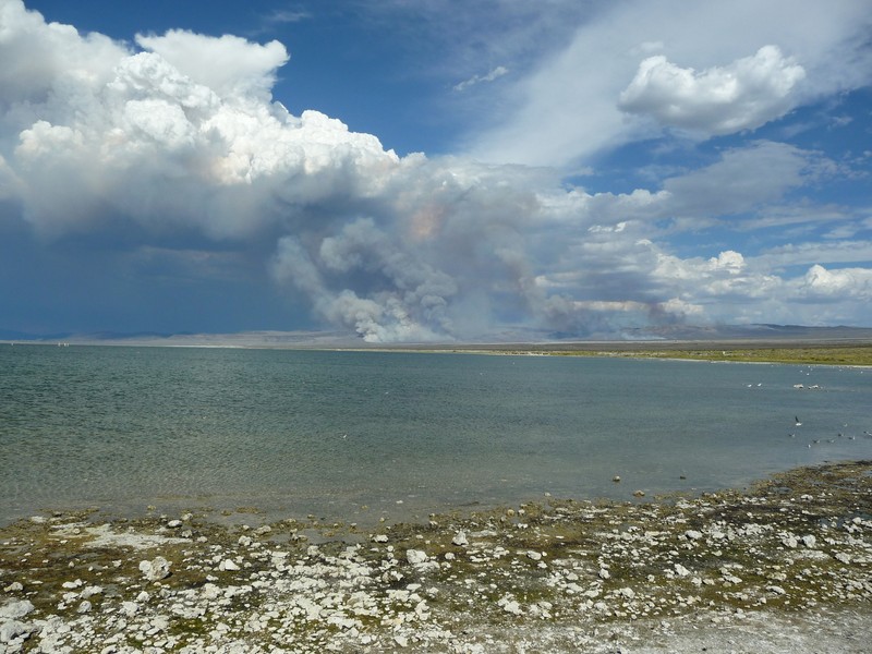
Smoke aerosol feeding a convective cloud system over Mono Lake, California. Image from EGU Imaggeo image repository and is provided by Gabriele Stiller.

One of the key messages for me was his conclusion that there has been substantial improvements in our understanding of aerosol and cloud processes since the previous IPCC report in 2007 but that this ‘knowledge’ hasn’t quite made its way into current global climate models. As someone who works on understanding aerosol processes from observations of the ambient atmosphere, this is something I very much agree with!  The implication here is that aerosol uncertainty will reduce in the future as this knowledge is translated to future climate models. We can but hope.

Some of the other key points from his talk included:

  1. Confidence in satellite based global average aerosol optical depth trends is low.
  2. Black carbon dominates uncertainty in aerosol radiative forcing.
  3. Many gaps in understanding including absorption by black carbon, trends and circulation changes due to aerosol forcing.
  4. Low level clouds are the “joker in the pack” of cloud feedbacks as they are the least understood area for clouds.

Still plenty of work to do!

Emission reductions

The short-lived climate forcers session in the afternoon included a very nice study of how emission regulations in California have affected air pollutant emissions, including black carbon. Tom Kirchstetter presented measurements of trucks using the Oakland port just across the bay from the AGU venue in San Francisco. The neat thing about the study was that this was done over several years both before the regulations were in place and afterwards. The regulations required diesel particle filters to be installed in new trucks, while old trucks had to be retro-fitted with them.

These new regulations have seen an 80% decrease in black carbon emissions over 4 years. The reduction is about 5-times faster than ‘natural’ fleet turnover, which occurs more gradually as new vehicles with improved engines replace older models. The new rules apply to 10,000-20,000 vehicles and will likely significantly improve air quality in the area. Further regulation will soon come into force for 1 million buses and trucks, which could have profound impacts on black carbon emissions in California.

This will likely be an interesting area to keep an eye on in terms of the wider potential impacts on air quality and climate.

AGU 2013 day 1: Short-lived climate forcers

My first day at AGU 2013 revolved around sessions on short-live climate forcers, which are components in the atmosphere that have short lifetimes (compared to carbon dioxide for example) and generally warm the atmosphere. Reduction of these compounds, such as methane and black carbon, has been mooted as a way to reduce global mean temperatures in coming decades.

This is summarised in the figure below, where the modelled impact of reducing black carbon and methane alongside reductions in carbon dioxide emissions are shown. The majority of the benefit in reducing methane and black carbon is felt by 2040 – if you look at longer time scales, then the effect diminishes relative to carbon dioxide.

image

Modelled impact of various reductions in carbon dioxide, methane and black carbon (BC) on global mean temperature. Figure courtesy of UNEP Integrated Assessment of Black Carbon and Tropospheric Ozone.

The problem with this idea is that there is much uncertainty related to these short-lived components, so it isn’t clear how much global temperatures would respond to a reduction in their atmospheric concentrations. This is represented in the above figure by the vertical bars to the left of the graph – there is much overlap here, which reflects this uncertainty. The health benefits of reducing black carbon in particular are quite clear though. Most of the talks focussed on black carbon and that is what I am also going to focus on below.

Fuzzy metrics

Tami Bond made some excellent and thought-provoking points on how short-lived climate forcers are framed relative to carbon dioxide. The key property for black carbon in the framework of near-term reductions in global temperature is its short lifetime in the atmosphere (days-to-weeks). This means that it is not evenly distributed across the globe, unlike greenhouse gases such as carbon dioxide and methane. This results in its radiative forcing being spatially distinct – the perturbation it has on our planets energy balance occurs close to its source of emission. The impact of such changes is usually felt more at the regional level, rather than the global scale associated with carbon dioxide. Her main point was that this is then an apples-to-oranges comparison, so for example, reducing black carbon emissions in Asia might not have a great impact of global mean surface temperatures but it may well reduce temperatures in the region and slow the effects of carbon dioxide driven warming.

She also reiterated the difficulties associated with the pollutants that are co-emitted with black carbon, which complicate the picture and are one of the major reasons that there is substantial uncertainty surrounding reducing black carbon. In the real world, you can’t really just reduce black carbon – any technological  solution will likely perturb the other pollutants, which tend to cool our climate. Attempts to reduce black carbon might actually result in temperatures rising – I’ve written more on studies that have considered this here.

Other highlights

Yi Deng presented a fascinating study of how aerosol particles can influence the atmosphere far away from their actual location by modelling the impact of biomass burning in Southern Africa on the Asian Summer Monsoon. He showed that the substantial burning that occurs actually strengthens the monsoon by inducing circulation changes up-wind of the Indian sub-continent and south-east Asia. We tend to think of aerosol impacts being confined to their atmospheric location but this illustrated how joined-up our atmosphere is.

One of the issues with black carbon is that some sources have received little attention previously. Ed Fortner from Aerodyne Research Inc. presented measurements of emissions from brick kilns in Mexico, which produce a lot of black carbon. There are around 300,000 kilns worldwide producing 1.5 billion bricks per year! Over half of these are in China (54%), with India (11%), Pakistan (8%) and Mexico (7%)  being the other major kiln hotspots. Characterising the emissions from these and other sources is likely going to be in important for efforts to constrain the impact of black carbon on both our climate and health.

Chris Cappa presented follow-up work to his 2012 paper in Science that investigated how much warming by black carbon is enhanced by other aerosol species that coat it. Black carbon warms the atmosphere by absorbing sunlight and both laboratory and theoretical evidence suggests that this is increased by coatings on the black carbon particles. This coating focusses sunlight onto the black carbon core, like a magnifying glass held to the sun does and this increases the absorption by the black carbon, a phenomenon known as “lensing”. Chris has been busy testing how much enhancement we see in the real world using measurements and typically to enhancement ranges from 10-30%, which is lower than is often suggested by aerosol models. There are significant caveats here as the measurements are challenging and require the aerosols to be “dry” – this is important as water often condenses onto aerosol particles and increases their reflective and lensing ability. This could be a vital ingredient in this process and it is a significant challenge to overcome.

My final highlight was presenting my poster! The AGU poster hall is absolutely massive and must span several football pitches. Despite this, the sessions are hugely rewarding and are a great opportunity to discuss science with a variety of people. The posters are a major part of the AGU fall meeting, which is not always true of other conferences. I’m looking forward to roaming the hall now that my own poster is done.

Me presenting my poster on day 1 of AGU 2013. Image courtesy of Sam Illingworth.

Me presenting my poster on day 1 of AGU 2013. Image courtesy of Sam Illingworth.

Communicating uncertainty

With all this complexity revolving around black carbon and the interest it has received from policy makers, Tami Bond was asked how to communicate this to non-scientists. Her response was:

Keep it simple but don’t ignore physical reality.

That seems like a pretty good mantra to me.

A continent on fire

While preparing my poster for the upcoming AGU Fall Meeting, I downloaded some data on fire activity in South America for background on why we are interested in biomass burning in the region. I wanted to quickly check I had the data in the correct format, so I just plotted the coordinates of the fire counts without an outline of South America.

I was surprised to see that the fire locations for August-October 2012 did a great job of outlining South America on their own!

Fire map.

Map of fire locations during August-October 2012 in South America from MODIS data from the Terra and Aqua satellites provided by NASA’s Earth Observing System Data and Information System (EOSDIS).

The data is from the MODIS instrument on NASA’s Terra and Aqua satellites. The data reports fire locations based on measuring  the emission of infrared radiation by the land surface from space (like the infrared cameras on your favourite police chase tv show).  Any 1km pixel with a fire detected within it is then included in the data – there could be more than one fire within the pixel but the instrument can’t distinguish these. You can find out more information about the technique here.

The widespread nature of the burning across South America is striking. Huge areas of the continent have fires detected within them. This is an annual endeavour with many of the fires started by people for land use change and agriculture. The main “season” runs from August to October, with the peak usually in September. These fires have been occurring for several decades now and they have transformed vast swathes of South America.

The burning produces large amounts of smoke, which can build up and pollute our atmosphere. This has important consequences for regional and global climate, air quality and also ecosystem development. I’m part of a project called SAMBBA, which as well as being a great acronym, is attempting to address some of the aspects of biomass burning that we don’t understand (which is a long list). I’ve written about the project and my part in it here and here previously.

As the map above illustrates, it is quite a big deal in the region. Stay tuned for future updates on the project.

Spoiling the view

Probably the most obvious manifestation of air pollution comes when looking out of the window and scanning the horizon – does the landscape go on for miles or is the view reduced? The build-up of air pollution can often dramatically reduce visibility via a shroud of haze.

On a recent trip to the Turkish Mediterranean coast near Antalya, the impact of air pollution on visibility was abundantly apparent. Below are two photographs I took of the view.

View of

View of the Beydağları Mountains in Antalya Province, Turkey. The top image is from the morning of 11th November 2013, while the bottom image is at sunset on the 12th November 2013. Photographs by Will Morgan (me).

The photographs look out to the west from the hotel I was staying in. In the top picture, there is little to see aside from a few tall buildings just observable beyond the trees in the foreground. In the bottom image though, the Beydağları Mountains can be seen, although the view is still hazy. The mountains were approximately 20 miles (32 km) away, so to not be able to see the mountains at all in the top picture requires a large amount of haze. During the ten day trip, views like the top image were far more common.

Antalya province is surrounded by the Taurus Mountains, with the Mediterranean sea to the south, so it forms a bowl-like basin where air pollution can build. It is also very sunny, which gives atmospheric chemistry an extra kick to form air pollution. This cocktail is similar to other pollution hotspots such as Mexico  City and Los Angeles.

The other key feature is that temperature inversions are common in Antalya. Typically, the temperature cools in the lowest part of the atmosphere with height but these inversions see a reversal of this trend within the first few hundred metres, which prevents air rising and mixing efficiently. You end up with a basin with a lid on it, so when pollutants are emitted into this, they find it difficult to disperse. This is like mixing a squash or cordial with water and only filling the glass half way with water – the amount of cordial (pollutant emissions) remains fixed but the reduced water level (temperature inversion) sees the concentration rise. Below is a video of a demonstration of temperature inversions, which actually refers to air pollution in Denver.

Click here to display content from YouTube.
Learn more in YouTube’s privacy policy.

The apparent major source of air pollution in Antalya is the burning of low-quality coal and domestic wood burning, which is particularly prevalent during the winter. I also noticed small fires from agricultural and trash burning during my stay. Summer temperatures typically exceed 30°C, so air conditioning is common rather than central heating systems. Evening and overnight temperatures during the winter drop below 10°C, so some form of heating is required.

The impact of air pollution on visibility is clear in the region and the health implications are also known, with Doctors warning about the risk from air pollution. Just this week, there were news reports warning that Antalya would experience poor air quality this winter.

Tackling the challenge is not easy though, especially given that the geographical and meteorological conditions in the region can’t be controlled. Antalya illustrates the interplay between these natural factors and our own role in pollutant emissions, which presents particular difficulties when trying to improve air quality. This interplay is prevalent across the globe.