My first day at EGU 2014 in Vienna was principally spent listening to various speakers describe the life and death of tiny particles in the atmosphere, known as aerosols. These aerosol particles come from a variety of sources – one of the major sources is through burning of fossil fuels, which produces a cocktail of pollutants that form these particles. They can also arise from natural sources, such as bursting bubbles on the ocean surface, strong odours from trees and high winds whipping up sandstorms in the desert.
Pinning these sources down is tough but we also have to understand how they evolve in the atmosphere from their birth, their growth during their adolescent years and ultimately their adult years, where they can influence our climate and health. At some point, they are removed from the atmosphere where they become an ex-aerosol. Understanding these different changes is necessary if we are going to be able to understand their impact both in the past, present and future.
Baby steps
One of the major routes for an aerosol to be born is via ‘nucleation’ where the particles form tiny clusters, which are around 100,000 times smaller than the width of a human hair. These clusters form due to the combination of different gas phase molecules, which given the right cocktail and conditions, can condense to form these initial tiny particles. I’ve previously written about these early steps here.
There was work presented here at the EGU by Jasmin Tröstl from the Paul Scherrer Institute in Switzerland showing that chemical species known as oxidised organics take part in this initial process. The abstract for the work is available here.
For a long time, sulphuric acid was thought to be the vital ingredient for this nucleation process but recent work at a laboratory at CERN (known as the cleanest box in the world) has illustrated the importance of several other species. You can read more about two studies in Nature that were published in the past few years on these here and here. Oxidised organic species are abundant in the atmosphere, so it isn’t a huge surprise that they are important but it has only been through the development of the new laboratory at CERN and sophisticated new instrumentation that the importance of this key ingredient has been demonstrated.
The difficult years
The same study also illustrated that these oxidised organic species were vital for the growth of these nucleated particles. This is the key stage for such particles as they essentially either grow or suffer an early death. When they start out, they are too small to become cloud particles, which is their main route to impacting our climate. So without growing they will never know the wet embrace of a cloud droplet.
Not only did the oxidised organics strongly increase the growth of these particles but their addition was enough to reconcile the laboratory measurements with observations of the real world. This is an enlightening step as it has previously proven difficult to mix up the right cocktail to represent what really goes on in the atmosphere, which suggests a deficit in our knowledge of this important process.
All grown up
Once they reach adulthood, these particles become important from a human health and climate perspective. They can build-up in the atmosphere over a matter of hours or days and influence our lives.
Rongrong Shen from Karlsruhe Institute of Technology, Germany, presented measurements of spring time pollution in Beijing during 2012, focusing on the chemical makeup of the pollution. Her abstract is available here. Beijing is well known as a hotspot for pollution, with over 20 million people living in the city and over 5 million vehicles on the road frequently creating a heavy chemical soup. The average concentration for PM2.5 (aerosol particles with a diameter less than 2.5µm) was 89µg/m3, which is far in excess of what is considered healthy. Even the ‘clear’ days in terms of visibility saw average concentrations of around 45µg/m3 . The World Health Organisation guidelines recommend the daily average values should remain below 25µg/m3, while annual values should be 10µg/m3 or lower.
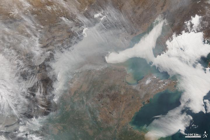
Haze over Beijing and surrounding region from 22 March 2007. Image credit: NASA Earth Observatory
More severe pollution episodes were typically driven by species such as sulphate and nitrate, which are known as ‘secondary’ species. This means that they start out as a gas and then condense onto pre-existing aerosol, such as nucleated particles or direct emissions from car exhausts and other forms of combustion. The results also indicated that such episodes were not solely driven by emissions within the city; the wider region played a role, including industrial sources and other Chinese cities. This is a common feature of pollution episodes in Western Europe also, which I wrote about recently here and here.
This is an ex-aerosol
Urs Baltensperger from the Paul Scherrer Institute, Switzerland gave the Vilhelm Bjerknes Medal Lecture and included a discussion of the fate of aerosols in the atmosphere. His abstract is available here. Aerosols are typically removed from the atmosphere via crashing into something, such as the ground, or by forming cloud droplets. These cloud droplets either evaporate, leaving an aerosol particle behind or they can grow to form rain, which removes the aerosol from the atmosphere. The rainfall can also washout other aerosols by catching them on the way down.
He referred to several previous studies, including measurements very early in the aerosol life cycle in an urban environment (Paris) and more mature aerosol at a high altitude site in the Swiss Alps at the Jungfraujoch.
The urban study illustrated that aerosol particles are quite diverse in this environment, which affects how readily they would form cloud droplets. Black carbon is known to be a poor candidate for making a cloud droplet, which the study showed. However, the results also illustrated that adding some other chemical components to the mix can vastly increase the likelihood of the particle joining the cloud droplet gang. This is important as the removal of black carbon from the atmosphere is poorly understood and can have significant implications when trying to predict its climate impact.
At the high altitude site at ‘the top of Europe’, the aerosol properties are more uniform. This makes it somewhat easier to predict how many particles will form a cloud droplet. This is an important result for models of aerosol impacts, as such a situation is more reflective of the scales that atmospheric models work in, particularly for climate change studies. This result is not true everywhere though, so as aerosol scientists we need to work towards understanding the differences across the globe, so that we can understand the ultimate fate of aerosol particles.

Image of the Swiss Alps during a research flight on the FAAM BAe-146 research aircraft. Photo credit: Will Morgan
That concludes this diary in the life of an aerosol particle; they have a hard and complex life, which often lasts just a few days or maybe weeks.
I’ll be back with more later this week.
—————————————————————————————————————————————————————–
Edit 03/05/14: Urs Baltensperger was originally spelt incorrectly.