Groundwater

Bubbling Merrily: Artesian Springs

Matt Herod December 7, 2015

Click here to display content from www.youtube.com

Always display content from www.youtube.com

I recorded the video above on a recent field camp near Deep River, Ontario. This video shows a great example of a flowing artesian spring which is bubbling up at the headwaters of a creek. The water is freezing, crystal clear and totally delicious! The classic textbook on groundwater, Freeze and Cherry, puts the attraction of groundwater springs nicely when they say “Flowing wells (along with springs and geysers) symbolize the presence and mystery of subsurface water, and as such they have always evoked considerable public interest.”

There are two types of artesian springs. Those that are controlled geologically, which are commonly taught as the only variety of artesian system, and topographically, which are often overlooked.

Geologically controlled artesian springs/wells result from a specific combination of hydrogeologic conditions. Specifically, the aquifer must be under pressure, which is usually caused by a steep elevation gradient in combination with relatively impermeable confining layers such as clay. This is called a confined aquifer. Recharge to this aquifer occurs on top of a hill, where the aquifer outcrops. This water then infiltrates through the permeable sediments to the water table and into the confined aquifer. However, this does not explain why a spring or a well drilled into and artesian aquifer often bubbles up with water, like the video above.

A conceptual model of a confined artesian aquifer in which the recharge area is exposed at higher elevation and the aquifer sediments are bounded by two aquitards. Source

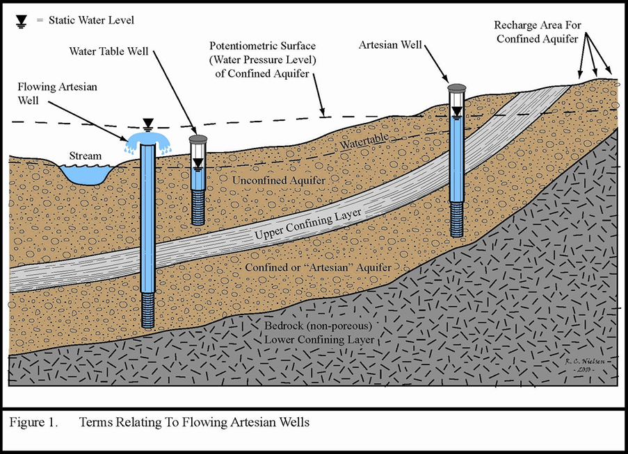
The reason for this is somewhat abstract and has to do with water pressure. In an unconfined aquifer the water table and the potentiometric surface, which is the abstract line dictated by the water level in the well, are generally synonymous and are defined by the point at which the water pressure is equal to atmospheric pressure. However, in confined aquifers where artesian conditions exist this becomes more complicated. The reason for this is that within the confined aquifer the water pressure is often greater than atmospheric. Imagine diving down in a lake and feeling the pressure of the water above you. Therefore, when this aquifer is drilled or a pathway to conduct water to the surface exists the water will want to flow upward towards that point where the water pressure and the atmospheric pressure are equal. This point can be above the ground surface and this leads to flowing artesian conditions. The figure below illustrates this concept nicely.

Source: Minnesota Department of Health,

In this figure the water level in the well on the right, which is connected to the confined aquifer, is distinct from the water table in the unconfined aquifer. The water is not flowing because the potentiometric surface is not higher than the ground level. In the other artesian well, which is flowing, the water flows up to the potentiometric surface, well above the ground surface. This is because that surface represents the point where the water pressure, which is the pressure of the water within the confined aquifer, and the atmospheric pressure are equal.

The other type of artesian spring are topographically controlled and often occur in valleys. The reason for this is that as water recharges at the top of hills this can locally raise the potentiometric surface if there is a steep valley nearby. Therefore, at the base of the valley the potentiometric surface can be higher than the ground surface causing water to discharge.

So which type is the one in the video? Let’s start by checking the topo map of the region. The spring is located at the red star, which based on the terrain map is actually pretty flat, certainly much flatter than the opposite bank of the Ottawa river.

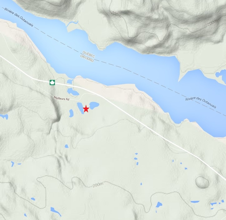
Based on this map it doesn’t look like the spring is topographically controlled. There may be some local elevation that does not show up at the map scale, although I don’t recall there being that much. One thing to keep in mind about this location is that there is a lot of bedrock exposed. It is possible that some of this bedrock aquifer is over-pressured and water flowing through fractures in the bedrock is discharging as a flowing artesian spring. In my mind, after about 10 minutes of looking around, this is the most likely scenario. It may also be completely wrong, but without a more detailed look around it is difficult to say.

Artesian springs and springs in general really represent the importance of protecting our groundwater resources. It is critical that places such as this artesian spring be protected from contamination and development as they are very fragile and represent important sources of clean, safe water as well as habitat to a large diversity of local flora and fauna. If you know of any artesian springs in your area please comment below and let me know if they are protected or if they have been compromised by contamination or development.

Matt

p.s. I’ve teamed up with Science Borealis, Dr. Paige Jarreau from Louisiana State University and 20 other Canadian science bloggers, to conduct a broad survey of Canadian science blog readers. Together we are trying to find out who reads science blogs in Canada, where they come from, whether Canadian-specific content is important to them and where they go for trustworthy, accurate science news and information. Your feedback will also help me learn more about my own blog readers.

It only take 5 minutes to complete the survey. Begin here: http://bit.ly/ScienceBorealisSurvey

If you complete the survey you will be entered to win one of eleven prizes! A $50 Chapters Gift Card, a $20 surprise gift card, 3 Science Borealis T-shirts and 6 Surprise Gifts! PLUS everyone who completes the survey will receive a free hi-resolution science photograph from Paige’s Photography!

ATTA and the Curious Case of Krypton-81

Matt Herod September 14, 2015

Ok, so I took some license with the title. This isn’t really a curious case and neither Krypton-81 nor ATTA are actually people. In fact, Krypton-81 (81Kr) is a radioisotope of the noble gas krypton and ATTA, which stands for atom trap trace analysis, is the revolutionary technique that has made its analysis possible. I recently heard about developments with ATTA at the IAEA Isotope Hydrology Symposium and have been doing some reading about the method and its revolutionary application to the dating of both young and ancient groundwater.

Figure 1. Dr. Z-T Lu working on the ATTA system at Argonne National Labs. Used with permission.

81Kr has long been a bit of a dangling carrot for groundwater dating people like myself. 81Kr is a long lived radioisotope of Kr (half-life: 229,000 years) that is produced by cosmic ray interaction in the atmosphere with other krypton isotopes. This production results in about 5 atoms of 81Kr for every 10^13 atoms of the other Kr isotopes. This 81Kr then settles to the earth surface and is incorporated into groundwater recharge and can then used to date groundwater from 150 thousand to 1.5 million years old. The way this works is that once water reaches the water table no new krypton is added and the clock starts ticking as the 81Kr decays away. In order to use this method we assume that the initial concentration in the recharge is in equilibrium with the concentration of 81Kr in the atmosphere, which is well mixed. ATTA then measures the amount of 81Kr that is left in the water sample compared to the other Kr isotopes and an age can be calculated from the difference between this ratio and the intial ratio.

ATTA can also be used for the short-lived isotope krypton-85 (half-life: 10.8 years). 85Kr is produced by fission in nuclear reactors and is released during nuclear fuel reprocessing. The short half life of 85Kr makes it useful for dating recently recharged groundwater from 1 to 40 years old.

Figure 2. Dating ranges of 85Kr, 39Ar, 81Kr and other established radioisotope tracers. (Source). Used with permission.

The reason krypton is such a useful tracer for groundwater dating is that as a noble gas the interaction of Kr with soils, rocks and the biosphere is minimal whereas other tracers such as 36Cl, 14C or 3H are often subject to retardation during transport or inputs from multiple sources which makes extensive corrections necessary or renders them completely unusable for dating. Furthermore, very few reliable tracers exist in the range that Kr isotopes cover making them extremely useful. One isotope that I haven’t mentioned as much is argon-39, which can be used to date water from 50-1000 years old, is also a noble gas, and can also be measured with ATTA.

Measurements of krypton can also be used for dating of ancient ice cores as well. Atmospheric gases including Kr are trapped in air bubbles in the ice and therefore, using the same method as groundwater dating, an absolute age for an ice core can be obtained. There are several other applications for Kr dating as well such as dating of deep crustal fluids and brines.

Figure 3. Sampling ice cores for Kr analysis by ATTA. Photo: V. Petrenko. Used with permission.

The development of atom trap trace analysis was first reported in Science in 1999 and since then has undergone several substantial improvements primarily aimed at reducing the required sample size required for an analysis of Kr. ATTA (Figure 4) works by trapping Kr atoms with a laser which causes a slight and temporary change in their atomic structure which lasts for about 40 seconds. During this period the Kr atoms in the laser beam are focussed and slowed and then trapped in an MOT (magneto optical trap) where they are held in place for an average of 1.8 seconds. Once the Kr atom is in the MOT it fluoresces as it returns to its original state. This fluorescence is detected by a camera which is sensitive enough to detect the emission from a single atom (Figure 5)!

Figure 4. Schematic layout of the ATTA-3 apparatus. (Source). Used with permission.

One of the key features of ATTA is that this laser induced fluorescence within the MOT occurs uniquely for every isotope as the laser frequency is tuned specifically! This means that only atoms of of the desired Kr isotope are trapped. Furthermore, this means that ATTA is completely immune to interference from other elements, isotopes, isobars, or molecules. In essence nothing can confuse the detection of the 81Kr atom once it fluoresces and therefore there is no background of spurious detections that need to be corrected for. Among low-level analytical techniques this is unique and a really big deal! As a user of AMS, which is another low level analytical method that does suffer from these issues, this is statement is an eye-catcher.

Figure 5. A CCD image showing the response of an atom in the MOT. Used with permission.

Since its invention ATTA has evolved considerably. We are now on the 3rd iteration of ATTA and significant improvements have been made that make ATTA much more practical for routine use. Specifically, the amount of sample required for an analysis has been reduced drastically. The first version of ATTA could only be used for atmospheric measurements as the quantity of Kr needed was too large to be extracted from water. ATTA-2 required ~1000 kg of water to extract 50uL of Kr gas. Now, ATTA-3 only requires 5-10uL of Kr which can be obtained from only 100-200 kg of water or 40-80 kg of ice. This advancement means that ATTA is now usable for groundwater dating applications never before possible. This has been demonstrated by the use of ATTA to date groundwater in Egypt to around 500,000 years old and even older water in Brazil up to 800,000 years. Other dating methods have confirmed that ATTA measurements are accurate.

Now that the sample sizes required for an 81Kr or 85Kr analysis have been lowered so dramatically the method is even more useful to the geoscience community. One of the messages from Dr. Lu’s talk at the IAEA meeting was that this technique is open for business and the geoscience community is strongly encouraged to reach out for collaboration and discussion. Furthermore, it may also be possible to use ATTA to measure argon-39, calcium-41 and potentially lead-205, strontium-90 and cesium-137,135 at extremely low levels.

Note: During the writing of this blog I corresponded with Dr. Z-T Lu, one of the creators of ATTA. I would like to thank him for allowing me to use his personal photos in this post. Dr. Lu is now establishing a radiokrypton dating centre at the University of Science and Technology of China.

References

Lu Z-T, Schlosser P, Smethie WM, Sturchio NC, Fischer TP, Kennedy BM, et al. Tracer applications of noble gas radionuclides in the geosciences. Earth-Science Rev. 2014;138:196–214.

Chen CY. Ultrasensitive Isotope Trace Analyses with a Magneto-Optical Trap. Science (80-). 1999;286(5442):1139–41.

Du X, Purtschert R, Bailey K, Lehmann BE, Lorenzo R, Lu Z-T, et al. A New Method of Measuring 81Kr and 85Kr Abundances in Environmental Samples. Geophys Res Lett. 2003;30(20):2068. Available from: http://arxiv.org/abs/physics/0311118

Aggarwal PK, Matsumoto T, Sturchio NC, Chang HK, Gastmans D, Araguas-Araguas LJ, et al. Continental degassing of 4He by surficial discharge of deep groundwater. Nat Geosci. 2014;8.

Lu Z-T. Atom Trap, Krypton-81, and Saharan Water. Nucl Phys News. 2008;18(2):24–7.

Guest Post: Jeremy Bennett – Approaches to modelling heterogeneity in sedimentary deposits

Matt Herod September 10, 2015

Hello everyone. Great that you could make it out to my blog post. I would like to introduce you to some ideas about environmental modelling that I have recently discovered during my work. These ideas are from this paper by Christine Koltermann and Steven Gorelick back in 1996. Whilst the primary focus of their paper is on modelling hydrogeological properties such as hydraulic conductivity, I think there is crossover with other modelling too.

What I find the most interesting about this work are the words they used to describe modelling approaches, meaning the way the modeller sees the world. They break down modelling into three different approaches: structure-imitating, process-imitating, and descriptive methods. Over the next few mousewheel-scrolls I hope I can explain these ideas in simple terms so that they are easy to understand.

This paper discusses models that are spatially distributed – this means that we are trying to estimate values at different locations in space. In the following diagrams I have simplified things to one dimension to hopefully make things a bit clearer. It is also important to note that many models will combine elements of one or more of the following model approaches – often at different scales.

Descriptive methods

Descriptive modelling approaches are primarily conceptual – kind of like joining the data dots in Figure 1 to produce the circle. There might be no hard and fast rules here, although models may be based on years of experience and observation in the field. These models may not be so rigorous and possibly difficult to replicate in different environments.

A good example of descriptive modelling are geological cross sections. They are constructed using borehole data and similar lithologies at similar depths are assumed to be part of the same geological formation. More experienced practitioners will have better intuition for connecting the dots and interpreting the stratigraphic record. In many cases thes cross sections are a suitable model. However in some hydrogeological applications this level of modelling is insufficient as more information is required about the geometry of the formation, and perhaps variations in its hydraulic properties – something that is difficult to derive solely from descriptive methods.

Structure-imitating methods

Structure-imitating modelling approaches quantify observations of the thing to be modelled and use these rules to produce something that looks similar. The structure that is imitated could be the actual shape of the object to be modelled, or it could be something more abstract, such as the geostatistical structure of the observations. To demonstrate: In Figure 2 we have some data shown with black lines. We can then derive information about this data, say in this case the distance of each data point from the centre. From this structural information we can model the rest of the circle.

A well-known structure-imitating method is kriging. This method uses the geostatistical structure (i.e. mean and covariance) of a set of observations to estimate values of a variable at other locations. A typical criticism of kriging and other geostatistical methods is that defined boundaries between facies become indistinct and don’t look so geologically plausible. Many other methods have been developed, such as multiple-point statistics, to address these arguments.

Process-imitating methods

Process-imitating modelling approaches rely on the governing equations of a process to produce a plausible model. Governing equations describe the physical principles underlying processes such as fluid motion or sediment transport. This type of approach can occur both as forward or inverse modelling. Forward models require setting key parameters in the model (such as hydraulic conductivity) and then predicting an outcome, such as the distribution of groundwater levels. Inverse models start with the observations and try to fit the hydrogeological parameters to the data.

Our final circle model is in Figure 3. In this particular case we know the equation that gives us the circle. As with all process-imitating modelling approaches there is some kind of parameter input required (or forcing). Here we have assumed that the circle is centred about the origin, and our parameter input is the radius of the circle (4) on the right hand side of the equation. Thus we can model the circle based on the equation and a parameter input.

The classic process-imitating model approach in hydrogeology is aquifer model calibration. This is a relatively simple, but widely used, application where zones of hydraulic conductivity are created and adjusted to reproduce measured groundwater levels (hydraulic heads). Often these zones are tweaked using a trial-and-error process to get a better match (or reduce the error). Aquifer model calibration is considered a process-imitating approach because it attempts to replicate the governing equations of fluid flow within porous media. MODFLOW is a model from USGS that is often used in this type of modelling.

Thanks for making it all the way down here. My aim was to provide you with a couple of new words to describe modelling approaches in geosciences and beyond. If you are working in hydrogeology then this paper by Koltermann and Gorelick is definitely worth a read – it gives an excellent foot-in-the-door to hydrogeological modelling.

Reference

Koltermann, C. E., and Gorelick, S. M. (1996). Heterogeneity in Sedimentary Deposits: A Review of Structure-Imitating, Process-Imitating, and Descriptive Approaches. Water Resources Research, 32(9), pp.2617-2658.

About Jeremy

Jeremy Bennett is conducting doctoral research at the University of Tübingen, Germany. He is researching flow and transport modelling in heterogeneous porous media. Prior to his post-graduate studies in Germany he worked in environmental consultancies in Australia and New Zealand. Jeremy figures there is no better way to understand a concept than to explain it to others – hopefully this hypothesis proves true. Tweets as @driftingtides and blogs here.

Geology Photo of the Week #46

Matt Herod August 27, 2015

This week’s photo brings us back to the world of geochemistry. I don’t have much information on this photo beyond that it was taken in Italy. However, if I may speculate a little it looks like these crystals may possibly be volcanic in origin and the fact that it was taken in Italy, which is famous for its volcanic sulphur deposits. I say this because such crystals are often found near active volcanoes and form from the degassing of sulphur dioxide (SO2) and hydrogen sulphide (H2S) gas from vents known as fumaroles. Groundwater dissolves gases and mineral rich in sulphur at high temperatures however, once the water reaches the low pressure atmosphere of the Earth’s surface these gases are released from the water and native sulphur precipitates.

Close-up of sulphur crystals with condensation drop by Ulrich Kueppers. Source