EGU Blogs

Black carbon

Aerosols and the pause

There is a new commentary piece in Nature Geoscience by Gavin Schmidt and colleagues on ‘Reconciling warming trends’. The paper investigates several potential causes for the discrepancy between climate model projections and the recent ‘slowdown’ in global surface temperatures, which is nicely illustrated on Ed Hawkins’ Climate Lab Book blog.

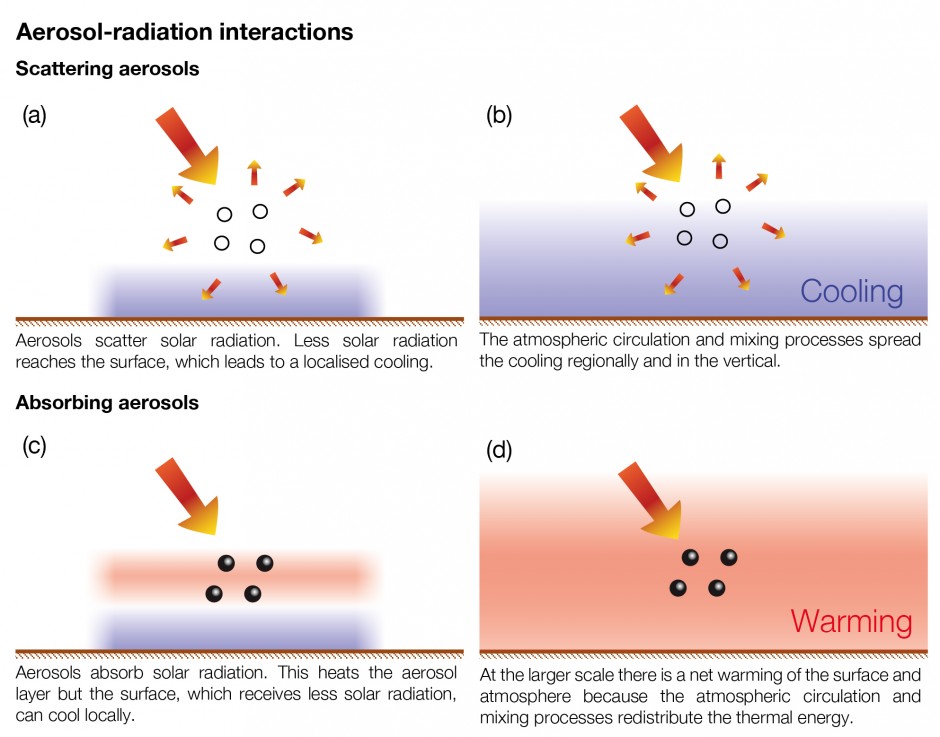
One of the aspects the paper looks at is the influence of aerosol particles in the troposphere (the lower part of the atmosphere), which tend to exert a cooling influence on our climate. Of the aspects they looked at, aerosol particles are the most uncertain.

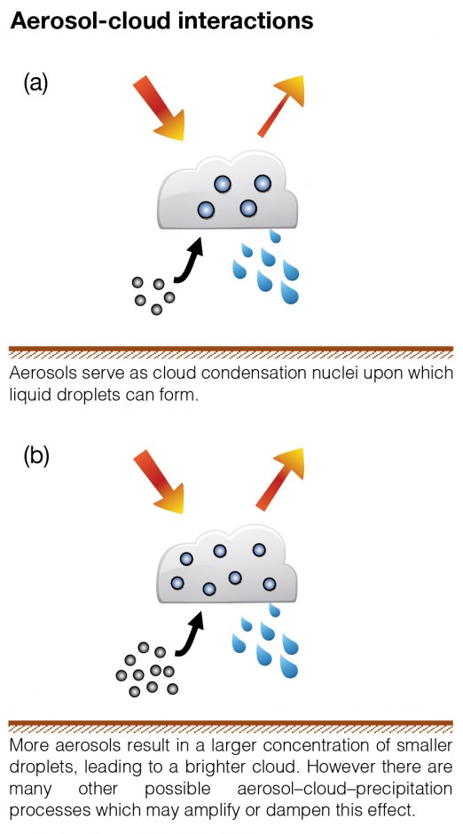
As I summarised in this previous post, the final report from the Intergovernmental Panel on Climate Change (IPCC) on the physical science basis concluded that aerosols was continue to dominate the uncertainty in the human influence on climate. They said that a complete understanding of past and future climate change requires a thorough assessment of aerosol-cloud-radiation interactions.

With this in mind, I want to delve into the details of how the chemical make-up of aerosol particles varies across the globe and how this is important for our climate and how this relates to the warming trends paper.

What are aerosols made of?

Aerosols are made up of a large variety of different chemical species, which vary by the time of day, seasonally, regionally and a host of other factors. There is no single type of aerosol in our atmosphere.

The figure below attempts to pull together a huge collection of studies that have been measuring the major aerosol chemical species in different regions of the globe. We can see on the map that many of the sites are in North America and Western Europe, where large coordinated surface networks have been making such measurements for decades. Measurements elsewhere are much more limited, particularly in the Southern Hemisphere.

This is one of the major difficulties in understanding aerosols; they are difficult to measure, the techniques used are typically quite labour intensive and they require access to well developed infrastructure and supporting measurements.

Fig7.13-Final-2

Summary of aerosol chemical species split across different regions based on surface measurements. The map shows the locations of the sites. For each area, the panels represent the median, the 25th to 75th percentiles (box), and the 10th to 90th percentiles (whiskers) for each aerosol component. The colour code for the measured components is shown in the key where SO4 refers to sulphate, OC is organic aerosol (strictly organic carbon), NO3 is nitrate, NH4 is ammonium, EC is black carbon (strictly elemental carbon), mineral refers to mineral dust e.g. from deserts and sea-salt refers to aerosols produced by ocean waves. The figure is 7.13 from the IPCC report, where the numerous references for the data are included. Click on the image for a larger view. Source: IPCC.

Bearing this in mind, we are able to draw some broad conclusions on their chemical make-up. We can see that in all of the non-marine regions, the aerosol is broadly made up of sulphate, organic carbon, nitrate, ammonium and black carbon, with the influence of mineral dust varying depending on location e.g. concentrations are much greater in locations such as Africa and Asia where large deserts exist.

Of these species, sulphate, nitrate, ammonium and black carbon are predominantly man-made in origin, while organic carbon can be a consequence of both natural and man-made emissions. We see that concentrations of organic carbon and nitrate are broadly equivalent to those of sulphate, with organic carbon being much greater in South America, Oceania, Africa and parts of Asia.

Where is the aerosol?

One of the key properties of aerosol particles in the troposphere is that they have a short lifetime, as they are removed from the atmosphere by rain or simply by crashing into things (terrible drivers those aerosol particles). This typically means that the largest concentrations occur near their sources; they are regionally very important in a climate context but their impact evens out at larger scales, although they do still exert a global influence.

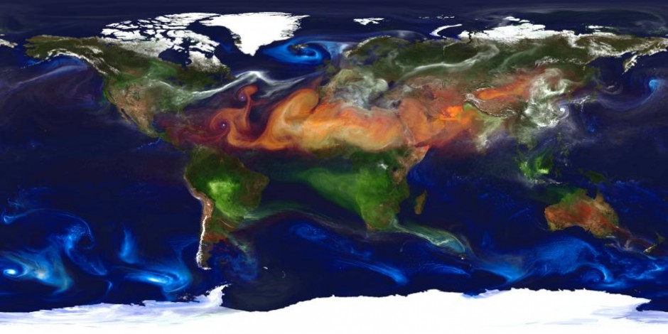
Below is an illustration of this based on satellite measurements combined with a forecast model system, which shows ‘hotspots’ of aerosol particles over China, India and Southern Africa in particular. The metric used here is the aerosol optical depth, which is a measure of the amount of aerosol present in a vertical slice through the atmosphere.

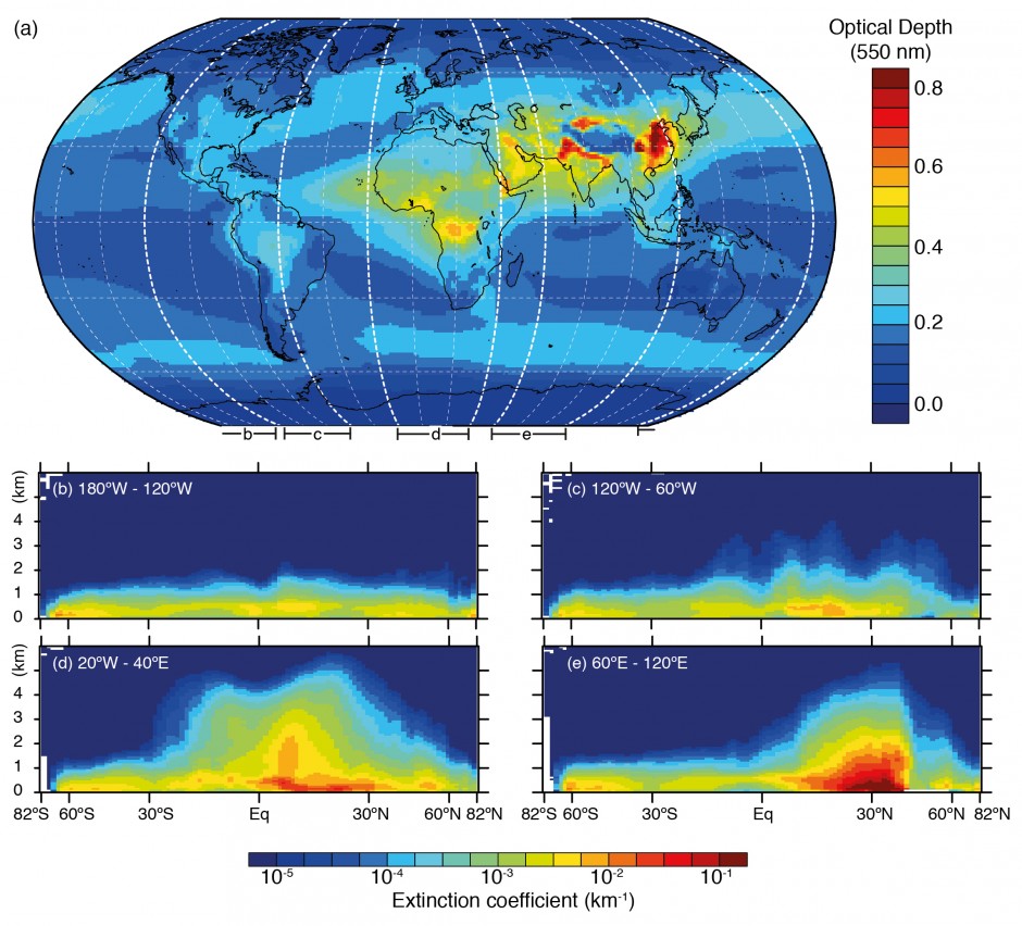
Horizontal and vertical distributions of aerosol amount based on a combination of the European Centre for Medium Range Weather Forecasts (ECMWF) Integrated Forecast System model with satellite measurements from the Moderate Resolution Imaging Spectrometer (MODIS) averaged over the period 2003–2010 and the Cloud–Aerosol Lidar with Orthogonal Polarization (CALIOP) instrument for the year 2010. The figure is 7.14 in the IPCC report and references for studies are available there. Click on the image for a larger view. Source: IPCC.

Comparing the two figures, we see that the enhanced aerosol optical depth in Asia is consistent with the large aerosol concentrations measured by the surface based networks. Of the man-made species, organic carbon is a big driver here, with nitrate, sulphate and ammonium also playing a major role. These aerosol particles are formed due to the substantial emissions from the region.

What about the pause?

Of these species, sulphate and black carbon are the major species that climate models have historically focussed on. Organic carbon is generally included, although there are large discrepancies in relation to measurements, particularly related to the secondary organic aerosol component. Nitrate has received comparatively little attention and those that have included it have shown that it is an important aerosol species both today and over the 21st Century. Drew Shindell and colleagues when comparing aerosol optical depth from satellite measurements and climate models concluded that:

A portion of the negative bias in many models is due to missing nitrate and secondary organic aerosol.

I’ve been involved in research showing how nitrate is important in North-Western Europe and how it enhances the aerosol radiative forcing in the region (many others have done so also by the way). Nitrate has long been known to be important in North America, particularly in California, where large urban and agricultural emissions coincide. Several studies have investigated its importance in East Asia, showing that it is particularly prevalent during the winter.

The ‘Reconciling warming trends’ commentary notes that nitrate was only included in two of the models that contributed to the Coupled Model Intercomparison Project (CMIP5) and that including this across all models brings them closer to the observed surface temperature trend. They also note that underestimating the secondary organic aerosol contribution would have a similar effect but don’t put a value on this.

While this certainly isn’t the last word on the importance of these species for climate change and research on the ‘pause’ will undoubtedly continue, further recognition of their contribution to atmospheric aerosol is a step in the right direction. There are many unanswered questions in this realm, particularly relating to the large differences across climate models in terms of what contribution each species makes to regional and global aerosol.

Bringing the aerosol measurement and modelling communities together more to address such issues is likely the way forward. This is a big focus in many aerosol related research projects these days…we’re trying, honest.

What did the IPCC say about aerosols?

Aerosols dominate the uncertainty in the total anthropogenic radiative forcing. A complete understanding of past and future climate change requires a thorough assessment of aerosol-cloud-radiation interactions.

This is one of the conclusions about aerosols and their impact on our climate from the the final report from the Intergovernmental Panel on Climate Change (IPCC) on the physical science basis that was released recently. What brought them to this conclusion and what does it mean? In this piece, I’ll go through the headline statements and findings.

The IPCC are concerned with assessing how various factors affect the Earth’s climate and it dedicates an entire chapter to aerosols and clouds, which is accessible here.

How do aerosols impact our climate?

Aerosols, can broadly influence the climate in two ways; aerosol-radiation interactions and aerosol-cloud interactions. The IPCC included some nice diagrams of how these processes occur, which I’ve included below.

Blah.

Illustration of aerosol-radiation interactions produced by the IPCC. This figure and more are available here.

Blah.

Illustration of aerosol-cloud interactions produced by the IPCC.

Both of these interactions are well established but the problem is pinning down the magnitude of these effects at larger scales and over time.

Headline numbers

The IPCC often refer to a term known as radiative forcing when assessing climate impacts. This illustrates the change in the amount of incoming versus outgoing radiation to our atmosphere. This regulates global temperatures and can affect things like circulation patterns and precipitation. Positive radiative forcing values increase temperature, while negative values reduce them. This value is usually referenced back to before the Industrial Revolution (typically 1750), when human influences on the composition of the atmosphere were more limited.

To put this in some context, the radiative forcing for carbon dioxide is 1.82 W/m2, with a reported range from 1.63 to 2.01 W/m2. What this means is that since 1750, adding carbon dioxide to our air has altered the radiation balance of the atmosphere and that this will cause a warming in the absence of any cooling factors.

In the table below, I’ve collated the various estimates for the aerosol influence from the report. As well as the central estimate, it is important to examine the range as this is one of the crucial aspects that drives the statements about our uncertain understanding of aerosols. The central estimates and the forcing range all suggest that aerosols exert a cooling influence on our climate; aerosols offset some of the warming influence from carbon dioxide and other greenhouse gases. If we first focus on the IPCC 2007 and 2013 values, we see that the central estimate has for the latest report (AR5)  indicates that aerosols are exerting less of a cooling effect than estimated previously. The range of the forcing estimate has also reduced.

The IPCC is effectively saying that the cooling influence from aerosols is slightly weaker than previously estimated and that our understanding has improved.

Blah.

Aerosol radiative forcing estimates.

The other values refer to different ways of calculating the impact and it is these numbers that inform the overall value in the report. The satellite based value refers to studies where satellite measurements of aerosol properties are used in conjunction with climate models; they are not wholly measurement based. In terms of studies using climate models on their own, the IPCC used a subset of climate models for their radiative forcing assessment, choosing those that had a “more complete and consistent treatment of aerosol-cloud interactions”.

The satellite based central value of -0.85 W/m2 is less negative than the central value from the climate models, which means the models indicate more cooling than the satellite based estimate. Compared to the subset of climate models that the IPCC used for their radiative forcing judgement, there is little overlap between their ranges also.

Why so uncertain?

This lack of agreement is a big driver for the large uncertainty range. It’s important to stress that there isn’t a strong reason to “trust” one set of results over another here as both satellite observations of aerosol properties and their representation in climate models are prone to many biases and it isn’t currently clear how these will impact the results.

Both methods are very sensitive to the assumed pre-industrial conditions assumed by the studies. Both methods have difficulties dealing with clouds but for different reasons.

Satellites can’t typically see through clouds, so they can miss aerosol trapped below them. Another major challenge is when layers of aerosol exist above clouds, which can affect the satellite measurements. Satellites are best suited to measuring the total amount of aerosol in the atmosphere. They have difficulty identifying different aerosol types, which means they can lump together natural and anthropogenic aerosols. They also have difficulty determining the relative importance of scattering or absorbing aerosols, which will determine the climate impact. Typically they can’t determine where the aerosol is in the vertical dimension of the atmosphere, which again will influence the climate impact. There are certainly advances in these areas but as ever, more work is required.

Models on the other hand, have difficulty representing aerosol-cloud interactions due to cloud systems typically being smaller than the resolution of a climate model, the complex number of processes at play and the lack of real-world measurements to test them. There is some evidence to suggest that climate models at the global scale tend to overestimate the size of the aerosol effect on cloud properties.

If we examine more details from the climate models, we see that there are large differences between models in terms of what types of aerosol it considers to be important. For example some models say that dust is a major contributor to the global aerosol burden, while others disagree. These are important details as climate models can sometimes broadly agree in terms of the radiative forcing estimate they provide but for very different reasons. Black carbon is another species that can contribute to varying degrees in different models, which is important as it warms the atmosphere; how a model represents black carbon is going to have a strong influence on the reported cooling. Nitrate is a potentially important species that often isn’t even included in climate models.

To summarise: it’s complicated.

What does this mean for climate change?

The short answer is: probably not a lot.

The change from the previous report is overall quite small (0.3 W/m2) and this is predominantly a result of improvements in our ability to represent aerosol processes (particularly clouds) since the last report. To put the change in context, between 2005 and 2011, the radiative forcing by greenhouse gases increased by 0.2 W/m2 due to increased concentrations in our atmosphere alone. At present, the uncertainties in aerosol radiative forcing mean that making definitive statements are likely unwise and putting faith in any one particular result will be fraught with difficulties. Focussing on the global scale also ignores the much larger regional impacts that aerosols can have, which is of more relevance to the wider issue.

The current state of understanding of aerosols suggests that they’ve exerted a cooling influence on our climate, which has offset some of the warming expected from the increase in greenhouse gases in our atmosphere. Improving this understanding will be crucial for assessing both past and future climate change.

AGU 2013 roundup

Now that the 2013 AGU Fall Meeting has ended, I thought I would roundup what I’ve been involved with over the week for both this blog and the Barometer Podcast, which I was recording each day with Sam Illingworth. Links to each piece are available below. Many thanks to all who have read and shared these over the past week.

Recording the podcast at conferences is becoming a trend as we’ve covered AGU now in 2012 and 2013 plus the EGU in 2013. Recording these is a lot of fun and particular thanks should go to Dave ToppingBethan Davies and Mark Brandon for giving up their time to chat to us this week. Lastly, many thanks to Sam for his infectious enthusiasm and for being the only person I’ve ever met with a louder laugh than me.

The conference itself was excellent throughout, even if the amount of science on offer was overwhelming at times. The sessions on science communication I attended were also fantastic, thought-provoking and often inspiring. I’m planning to write a separate post on this aspect over the coming days.

So long San Francisco! Image: Will Morgan

So long AGU 2013 and thanks for all the science! Image: Will Morgan

Blog posts

Podcasts

http://thebarometer.podbean.com/2013/12/10/fires-beer-and-satellites-day-1-at-agu/

http://thebarometer.podbean.com/2013/12/10/disappointment-aerosols-and-methane-burps-day-2-at-agu/

http://thebarometer.podbean.com/2013/12/12/hansen-nuclear-power-and-geologists-day-3-at-agu/

http://thebarometer.podbean.com/2013/12/13/science-communication-viscosity-and-londons-greenhouse-gases-day-4-at-agu/

http://thebarometer.podbean.com/2013/12/13/communicating-big-data-and-a-love-of-models-day-5-at-agu/

AGU 2013 Days 4 & 5: measurements & models

My fourth and fifth days at the AGU Fall Meeting involved dashing between multiple sessions to take in a number of talks on (surprise, surprise) aerosols! The main strand running through them from my point of view was how there are major efforts to construct large datasets of aerosol properties that can be used to test our understanding via numerical models.

Aerosols are complex and tend to stick around in the atmosphere for hours-to-weeks, rather than years-to-centuries. This means that they are spatially very diverse and also vary with time e.g. with the passage of seasons. This presents a challenge for our understanding but by constructing large datasets, it can also be used to constrain our numerical models.

For example, by looking at years of winter data for European pollution we might find that our models represent this quite well but it might be that there are significant errors when we look at the summer. This information is useful and might point us towards places to study further and improve our understanding. Just looking at a global annual average, this information is lost.

Image of the global aerosol distribution produced by NASA. The image was produced using high-resolution modelling by William Putman from NASA/Goddard. The colours show the swirls of aerosol particles formed from the numerous sources across the globe. The colours show aerosol particles as dust (gold/brown), sea-spray (blue), biomass burning/wildfires (green) and industrial/urban (white).

Image of the global aerosol distribution produced by NASA. The image was produced using high-resolution modelling by William Putman from NASA/Goddard. The colours show the swirls of aerosol particles formed from the numerous sources across the globe. The colours show aerosol particles as dust (gold/brown), sea-spray (blue), biomass burning/wildfires (green) and industrial/urban (white).

There were several talks detailing efforts to build satellite data sets of aerosol properties over long periods and use these to assess numerical models. Phillip Stier from the University of Oxford sounded a cautionary note by illustrating how different satellites can sometimes deliver different results for certain properties. He showed three different satellite images of cloud effective radius, which is a property of clouds that is important for how they interact with sunlight, and they were all very different. One of them agreed with his model but which set of measurements do you believe? He ended with a call to expand initiatives that seek to collate data from surface and aircraft measurements to test satellite measurements and models.

Dan Murphy from the National Oceanic & Atmospheric Administration paper presented some work on trends in aerosol over the past decade. He showed that while at a global level, the amount of aerosol in the atmosphere hasn’t really changed, it has changed significantly at the regional level. Aerosol concentrations have decreased in the USA and Western Europe, while they have increased in East Asia and in the Middle East. Aerosol has moved around a lot but there has not been a discernible change in their radiative effect at the global level. However, he said we couldn’t rule out that aerosols haven’t caused other adjustments such as circulation changes and clouds. You can access his Nature Geoscience paper on his work here. His work is consistent with several other papers that have shown negligible trends in global aerosol after the past decade.

These were highly interesting talks and should serve us well as we attempt to improve our understanding of aerosols, although there is much work still to do. No doubt we can anticipate much more work on this in the future – one of the talks did proclaim that:

Aerosol reanalysis is trendy.

No doubt we’ll be seeing the influence of this in the fashion houses of London, Paris and New York soon.